Layers

layer_id

Each layer requires a layer_id value. If you don’t supply one, it will create it for you, but this may have some unintended consequences for you.

The layer_id is the ID that deck.gl uses to ‘shallow-compare’ layers to see if they need updating. Which comes in handy when working in Shiny. If you update data, for example when using a reactive() function, and use the same layer_id, deck.gl knows it should update the layer rather than re-draw it completely.

However, if two of your layers of the same type have the same layer_id, then deck.gl will get confused and will only show the last layer drawn.

For example, if you have to scatterplot layers, both with the same layer_id, only the second one will be shown.

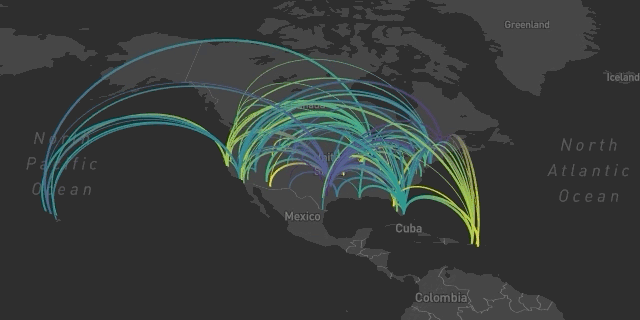
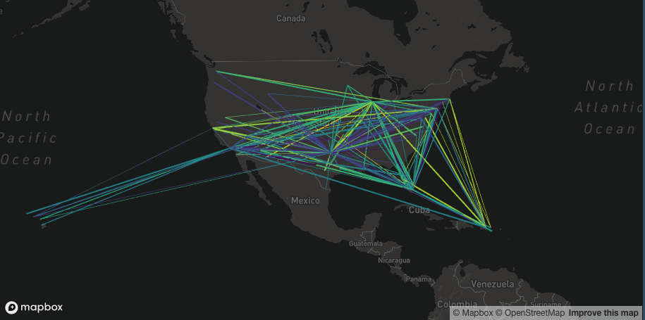
Arcs

url <- 'https://raw.githubusercontent.com/plotly/datasets/master/2011_february_aa_flight_paths.csv'
flights <- read.csv(url)
flights$id <- seq_len(nrow(flights))
flights$stroke <- sample(1:3, size = nrow(flights), replace = T)

mapdeck( token = key, style = mapdeck_style("dark"), pitch = 45 ) %>%
  add_arc(
    data = flights
    , layer_id = "arc_layer"
    , origin = c("start_lon", "start_lat")
    , destination = c("end_lon", "end_lat")
    , stroke_from = "airport1"
    , stroke_to = "airport2"
    , stroke_width = "stroke"
  )

Arcs

Animated Arcs

mapdeck( token = key, style = 'mapbox://styles/mapbox/dark-v9', pitch = 45 ) %>%
  add_animated_arc(
    data = flights
    , layer_id = "arc_layer"
    , origin = c("start_lon", "start_lat")
    , destination = c("end_lon", "end_lat")
    , stroke_from = "airport1"
    , stroke_to = "airport2"
    , stroke_width = "stroke"
  )

Arcs

GeoJSON

mapdeck(
  token = key
  , pitch = 35
  ) %>%
    add_geojson(
    data = geojson
    , layer_id = "geojson"
  )

GeoJSON

Great Circles

url <- 'https://raw.githubusercontent.com/plotly/datasets/master/2011_february_aa_flight_paths.csv'
flights <- read.csv(url)
flights$id <- seq_len(nrow(flights))
flights$stroke <- sample(1:3, size = nrow(flights), replace = T)

mapdeck( style = 'mapbox://styles/mapbox/dark-v9') %>%
  add_greatcircle(
    data = flights
    , layer_id = "arc_layer"
    , origin = c("start_lon", "start_lat")
    , destination = c("end_lon", "end_lat")
    , stroke_from = "airport1"
    , stroke_to = "airport2"
    , stroke_width = "stroke"
  )

Great Circles

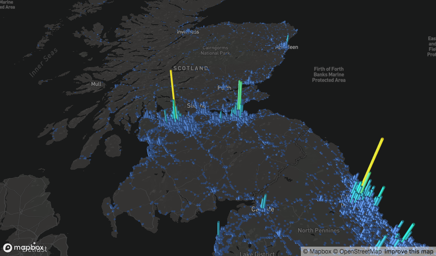
Grid

df <- read.csv(paste0(
'https://raw.githubusercontent.com/uber-common/deck.gl-data/master/',
'examples/3d-heatmap/heatmap-data.csv'
))

df <- df[!is.na(df$lng), ]

mapdeck( token = key, style = mapdeck_style("dark"), pitch = 45 ) %>%
add_grid(
  data = df
  , lat = "lat"
  , lon = "lng"
  , cell_size = 5000
  , elevation_scale = 50
  , layer_id = "grid_layer"
)

Grid

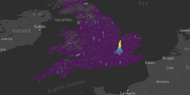
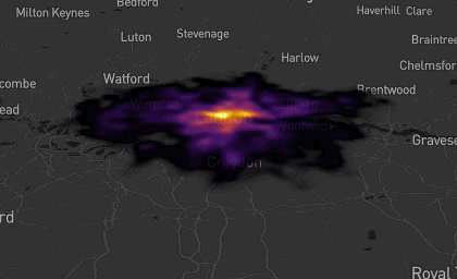
Heatmap

df <- read.csv(paste0(
'https://raw.githubusercontent.com/uber-common/deck.gl-data/master/',
'examples/3d-heatmap/heatmap-data.csv'
))

df <- df[!is.na(df$lng), ]

mapdeck( style = mapdeck_style('dark'), pitch = 45 ) %>%
 add_heatmap(
   data = df[1:30000, ]
   , lat = "lat"
   , lon = "lng"
   , weight = "weight",
   , colour_range = colourvalues::colour_values(1:6, palette = "inferno")
)

Heatmap

Hexagons


library(mapdeck)

set_token( read.dcf("~/Documents/.googleAPI", fields = "MAPBOX"))
df <- read.csv(paste0(
  'https://raw.githubusercontent.com/uber-common/deck.gl-data/master/examples/'
  , '3d-heatmap/heatmap-data.csv'
))

df <- df[!is.na(df$lng), ]

mapdeck( style = mapdeck_style("dark"), pitch = 45) %>%
  add_hexagon(
    data = df[ df$lat > 54.5, ]
    , lat = "lat"
    , lon = "lng"
    , layer_id = "hex_layer"
    , elevation_scale = 100
    , colour_range = colourvalues::colour_values(1:6, palette = colourvalues::get_palette("viridis")[70:256,])
  )

Hexagons

Lines

url <- 'https://raw.githubusercontent.com/plotly/datasets/master/2011_february_aa_flight_paths.csv'
flights <- read.csv(url)
flights$id <- seq_len(nrow(flights))
flights$stroke <- sample(1:3, size = nrow(flights), replace = T)

mapdeck( token = key, style = mapdeck_style("dark"), pitch = 45 ) %>%
  add_line(
    data = flights
    , layer_id = "line_layer"
    , origin = c("start_lon", "start_lat")
    , destination = c("end_lon", "end_lat")
    , stroke_colour = "airport1"
    , stroke_width = "stroke"
  )

Lines

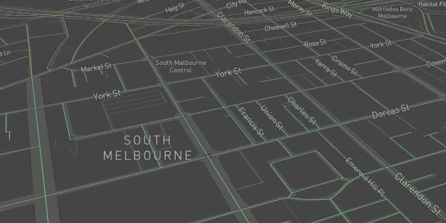
Path

mapdeck(
  token = key
  , style = mapdeck_style("dark")
  , zoom = 10) %>%
  add_path(
    data = roads
    , stroke_colour = "RIGHT_LOC"
    , layer_id = "path_layer"
  )

Path

Point cloud

df <- capitals
df$z <- sample(10000:10000000, size = nrow(df))

mapdeck(token = key, style = mapdeck_style("dark")) %>%
add_pointcloud(
  data = df
  , lon = 'lon'
  , lat = 'lat'
  , elevation = 'z'
  , layer_id = 'point'
  , fill_colour = "country"
)

Pointcloud

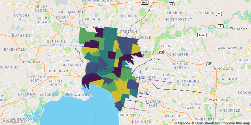
Polygons

library(sf)
library(geojsonsf)

sf <- geojson_sf("https://symbolixau.github.io/data/geojson/SA2_2016_VIC.json")
sf$e <- sf$AREASQKM16 * 10

mapdeck(token = key, style = mapdeck_style("dark")) %>%
  add_polygon(
    data = sf[ data.table::`%like%`(sf$SA4_NAME16, "Melbourne"), ]
    , layer = "polygon_layer"
    , fill_colour = "SA2_NAME16"
    , elevation = "e"
  )

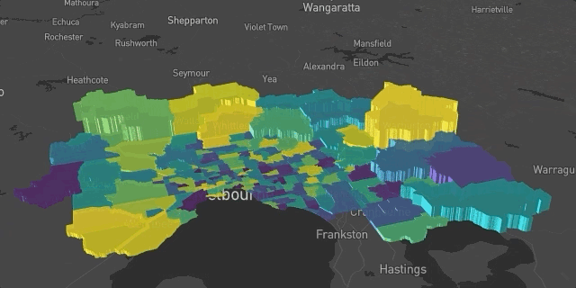
Polygons

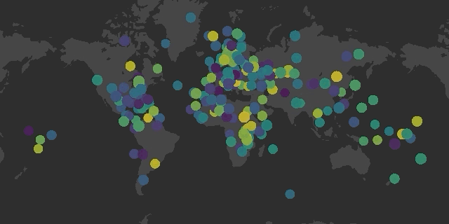
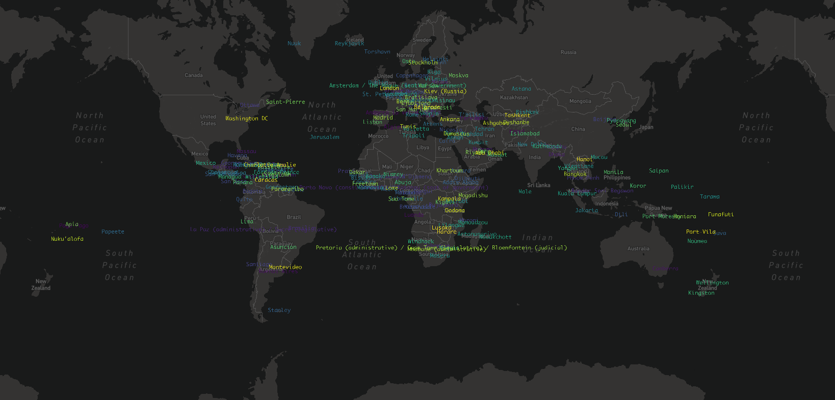
Scatter

mapdeck( token = key ) %>%
add_scatterplot(
  data = capitals
  , lat = "lat"
  , lon = "lon"
  , radius = 500000
  , fill_colour = "country"
  , layer_id = "scatter_layer"
  , palette = "plasma"
)

Scatter

Screen grid

df <- read.csv(paste0(
'https://raw.githubusercontent.com/uber-common/deck.gl-data/master/',
'examples/3d-heatmap/heatmap-data.csv'
))

df <- df[ !is.na(df$lng), ]

df$weight <- sample(1:10, size = nrow(df), replace = T)

mapdeck( token = key, style = mapdeck_style('dark'), pitch = 45 ) %>%
add_screengrid(
  data = df
  , lat = "lat"
  , lon = "lng"
  , weight = "weight"
  , layer_id = "screengrid_layer"
  , cell_size = 10
  , opacity = 0.3
  , colour_range = colourvalues::colour_values(1:6, palette = "plasma")
)

Screengrid

Text

mapdeck(token = key, style = mapdeck_style('dark')) %>%
  add_text(
    data = capitals
    , lon = 'lon'
    , lat = 'lat'
    , fill_colour = 'country'
    , text = 'capital'
    , layer_id = 'text'
    , size = 16
  )

Text

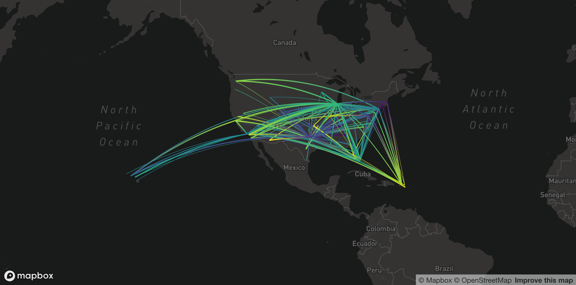
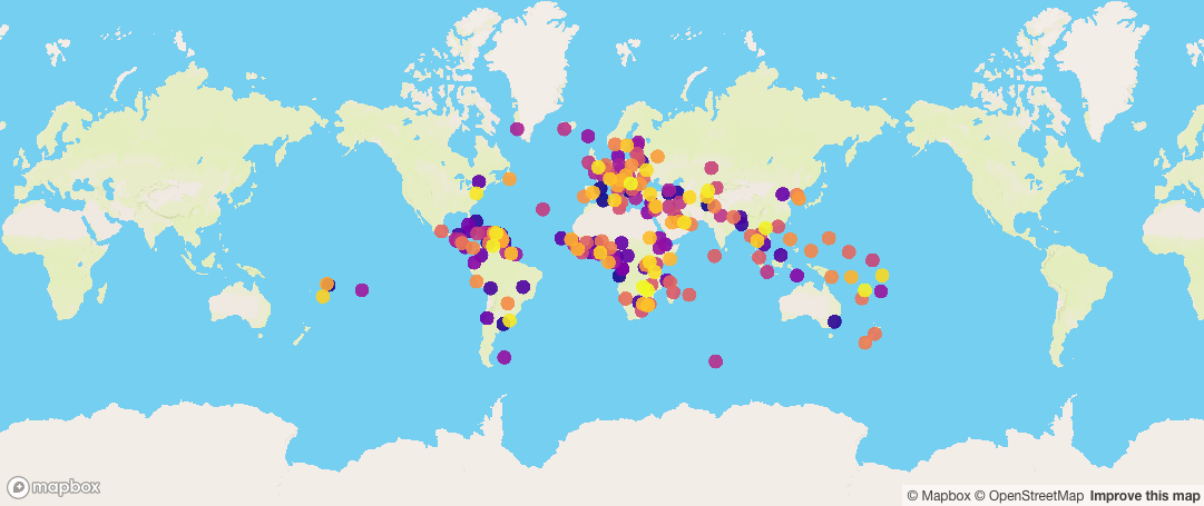
Multiple layers

df1 <- capitals[ capitals$country == "Australia", ]
df2 <- capitals[ capitals$country != "Australia", ]
df1$key <- 1L
df2$key <- 1L

df <- merge(df1, df2, by = 'key')

mapdeck(
  token = key
  , style = mapdeck_style("dark")
  , pitch = 35
  ) %>%
  add_arc(
    data = df
    , origin = c("lon.x", "lat.x")
    , destination = c("lon.y", "lat.y")
    , layer_id = "arc_layer"
    , stroke_from = "country.x"
    , stroke_to = "country.y"
    , stroke_width = 2
    ) %>%
    add_scatterplot(
    data = df2
    , lon = "lon"
    , lat = "lat"
    , radius = 100000
    , fill_colour = "country"
    , layer_id = "scatter"
  )

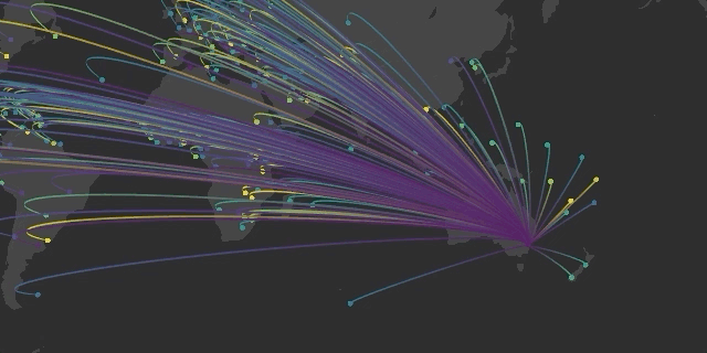
Multiple Layers

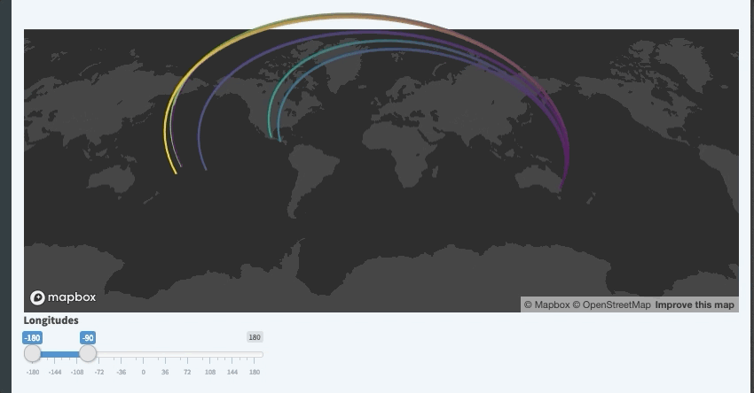
Shiny

The three main functions to use are

renderMapdeck() in the Server
mapdeckOutput() in the UI
mapdeck_update() to update an existing map

You can observe interactions with the layers by using observeEvent(). The event you observe is formed by combining

'map_id + "_" + layer + "_click"

where

map_id is the outputId of the mapdeckOutput() function
layer is the layer you’re interacting with
_click is you observing ‘clicking’ on the layer

There’s an example of this in the shiny.

library(shiny)
library(shinydashboard)
library(jsonify)

ui <- dashboardPage(
    dashboardHeader()
    , dashboardSidebar()
    , dashboardBody(
        mapdeckOutput(
            outputId = 'myMap'
            ),
        sliderInput(
            inputId = "longitudes"
            , label = "Longitudes"
            , min = -180
            , max = 180
            , value = c(-180,-90)
        )
        , verbatimTextOutput(
            outputId = "observed_click"
        )
    )
)
server <- function(input, output) {

    #set_token('abc') ## set your access token

    origin <- capitals[capitals$country == "Australia", ]
    destination <- capitals[capitals$country != "Australia", ]
    origin$key <- 1L
    destination$key <- 1L

    df <- merge(origin, destination, by = 'key', all = T)

    output$myMap <- renderMapdeck({
        mapdeck(style = mapdeck_style('dark'))
    })

    ## plot points & lines according to the selected longitudes
    df_reactive <- reactive({
        if(is.null(input$longitudes)) return(NULL)
        lons <- input$longitudes
        return(
            df[df$lon.y >= lons[1] & df$lon.y <= lons[2], ]
        )
    })

    observeEvent({input$longitudes}, {
        if(is.null(input$longitudes)) return()

        mapdeck_update(map_id = 'myMap') %>%
            add_scatterplot(
                data = df_reactive()
                , lon = "lon.y"
                , lat = "lat.y"
                , fill_colour = "country.y"
                , radius = 100000
                , layer_id = "myScatterLayer"
                , update_view = FALSE
            ) %>%
            add_arc(
                data = df_reactive()
                , origin = c("lon.x", "lat.x")
                , destination = c("lon.y", "lat.y")
                , stroke_from = "country.x"
                , stroke_to = "country.y"
                , layer_id = "myArcLayer"
                , id = "country.x"
                , stroke_width = 4
                , update_view = FALSE
            )
    })

    ## observe clicking on a line and return the text
    observeEvent(input$myMap_arc_click, {

        event <- input$myMap_arc_click
        output$observed_click <- renderText({
            jsonify::pretty_json( event )
        })
    })
}

shinyApp(ui, server)

Shiny

Layers

David Cooley

2020-08-17

Layers

layer_id

Arcs

Animated Arcs

GeoJSON

Great Circles

Grid

Heatmap

Hexagons

Lines

Path

Point cloud

Polygons

Scatter

Screen grid

Text

Multiple layers

Shiny