Core H3 Themes
Ray Shao, Sahinya Akila
2023-07-20
Source:vignettes/CoreH3Themes.Rmd
CoreH3Themes.RmdCore H3 Themes
There’s lots of really good content and documentation on the fundamentals of H3.
This post touches on some of the core concepts, and shows you how you
can use them in R through h3r
library(mapdeck)     ## Plots / Maps
library(sfheaders)   ## building sf objects
library(secret)      ## accesing Mapbox Token

mapdeck::set_token(secret::get_secret("MAPBOX"))
H3 is a geospatial indexing system that partitions the world into hexagonal cells
The H3 Core Library implements the H3 grid system. It includes functions for converting from latitude and longitude coordinates to the containing H3 cell, finding the center of H3 cells, finding the boundary geometry of H3 cells, finding neighbors of H3 cells, and more.
Cells
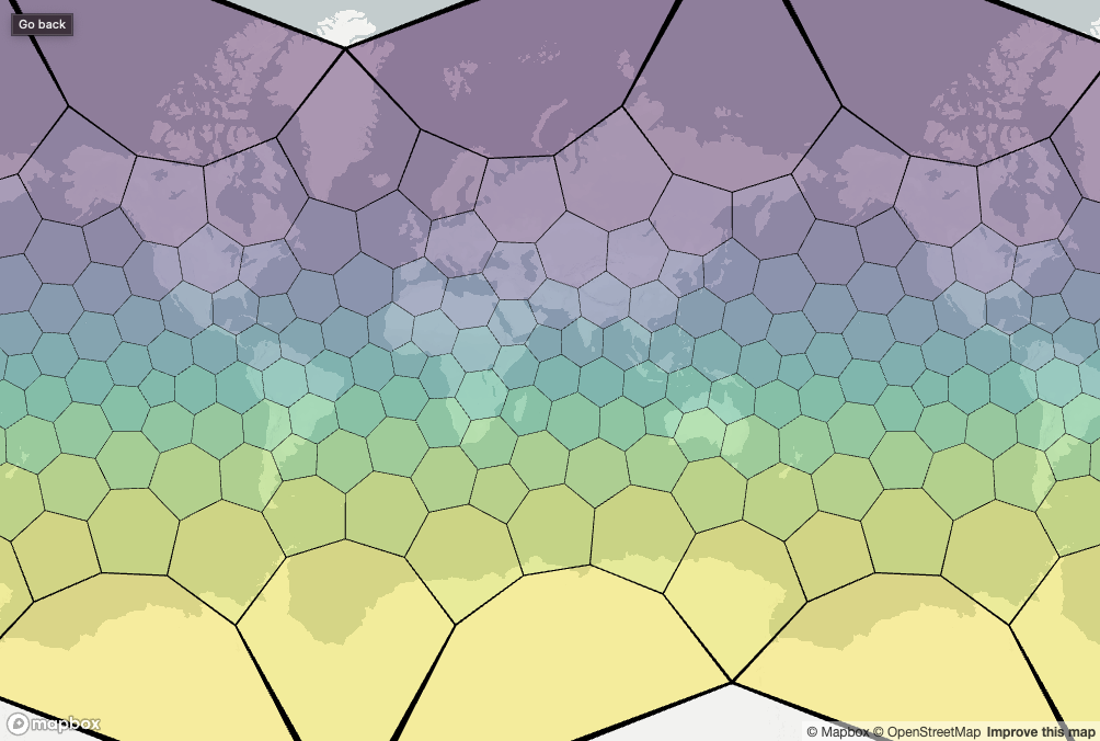
Resolution 0 cells are the largest (i.e, they cover the largest area) and resolution 15 are the smallest. The whole globe is covered with cells at each resolution.
We’re using the term ‘cells’ because each resolution is made up of some number of hexagons, and exactly 12 pentagons.
If we plot all the Resolution 0 cells on a ‘flat’ map we get distortions as the cells get further from the equator. This is purely a result of plotting using the Mercator projection. However, all hexagons at each resolution are roughly the same size.
cells <- h3r::getRes0Cells()
mapdeck(
  libraries = "h3"
  , style = mapdeck_style("light")
  , repeat_view = TRUE
  )  %>%
  add_h3(
    data = data.frame(x = cells)
    , hexagon = "x"
    , fill_colour = "x"
    , fill_opacity = 0.4
    , tooltip = "x"
    , stroke_colour = "#000000"
    , stroke_width = 25000
  )
Plotting (interlude)
We’re using the mapdeck library for the maps because it
uses deck.gl as the underlying plotting
engine. And given it is also developed by Uber, it can natively plot the
H3 Cells, so there’s no need to convert to lat/lon coordinates.
However, note that you have to tell mapdeck() you want
to plot the cells by adding the libraries = "h3"
parameter:
mapdeck(libraries = "h3") %>%
  add_h3()
Pentagons
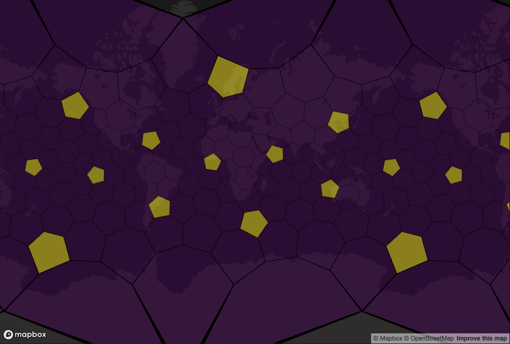
The reason for using pentagons is summarised by Uber
The H3 grid is constructed on the icosahedron by recursively creating increasingly higher precision hexagon grids until the desired resolution is achieved. Note that it is impossible to tile the sphere/icosahedron completely with hexagons; each resolution of an icosahedral hexagon grid must contain exactly 12 pentagons at every resolution, with one pentagon centered on each of the icosahedron vertices.
The nice feature about the pentagons is that they are all centered in the ocean.
cells <- h3r::getRes0Cells()
is_pentagon = h3r::isPentagon(cells)
mapdeck(
  libraries = "h3"
  , style = mapdeck_style("dark")
  , repeat_view = TRUE
  )  %>%
  add_h3(
    data = data.frame(x = cells, is_pentagon = is_pentagon)
    , hexagon = "x"
    , fill_colour = "is_pentagon"
    , fill_opacity = 0.5
    , tooltip = "x"
    , stroke_colour = "#000000"
    , stroke_width = 25000
  )
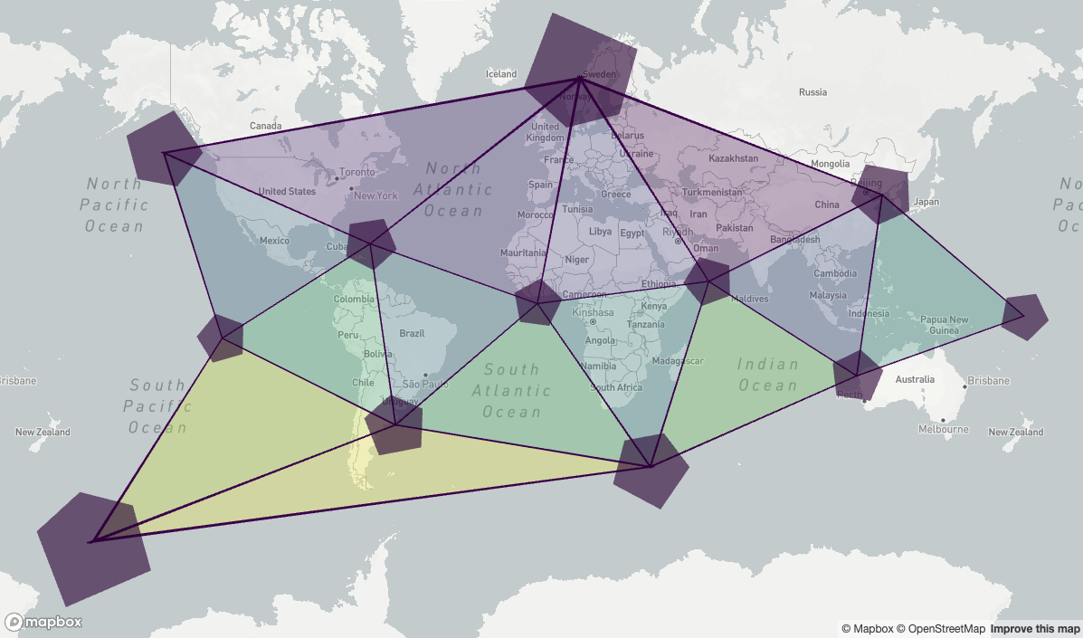
Icosahedron faces
And the pentagons are the corners of each of the 20 icosahedron faces (i.e, each triangle).
cells <- h3r::getRes0Cells()
is_pentagon = h3r::isPentagon(cells)

pentagonCells <- cells[as.logical(is_pentagon)]
pentagonFaces <- h3r::getIcosahedronFaces(pentagonCells)

## Make triangles out of the pentagons
df_pentagonFaces <- data.frame(
  cell = rep(names(pentagonFaces), lengths(pentagonFaces))
  , face = unlist(unname(pentagonFaces))
  )

df_pentagonFaces <- df_pentagonFaces[ order(df_pentagonFaces$face), ]

df_pentagonFaces <- cbind(
  df_pentagonFaces
  , h3r::cellToLatLng(df_pentagonFaces$cell)
)


sf_faces <- sfheaders::sf_polygon(
  obj = df_pentagonFaces
  , polygon_id = "face"
  , x = "lng"
  , y = "lat"
)
## For plotting reasons I'm removing the faces that cross the 180 & Poles
mapdeck(
  libraries = "h3"
  , style = mapdeck_style("light")
  , repeat_view = FALSE
  )  %>%
  add_polygon(
    data = sf_faces[ !sf_faces$face %in% c(1, 6, 11, 15, 16, 19), ]
    , fill_colour = "face"
    , fill_opacity = 0.3
    , tooltip = "face"
    , stroke_width = 50000
  ) %>%
  add_h3(
    data = data.frame(cell = pentagonCells)
    , hexagon = "cell"
    , fill_opacity = 0.6
  )
Changing Resolution
If we plot all the Resolution 0 cells at the center of each icosahedron face, plus the children of each of these (by going up to resolution 1) we see there are (approximately) 7 children per cell.
cells <- c(
  '8021fffffffffff', '8005fffffffffff', '800ffffffffffff', '8035fffffffffff',
  '803ffffffffffff', '8065fffffffffff', '8033fffffffffff', '8049fffffffffff', '8081fffffffffff', '8097fffffffffff', '8073fffffffffff', '805dfffffffffff',
  '808ffffffffffff', '80c1fffffffffff', '80abfffffffffff', '80bffffffffffff',
  '80b5fffffffffff', '80d3fffffffffff', '80effffffffffff', '80e5fffffffffff'
  )

children_cells <- unlist(h3r::cellToChildren(cells, 1L))
mapdeck(
  libraries = "h3"
  , style = mapdeck_style("dark")
  )  %>%
  add_h3(
    data = data.frame(x = c(cells, children_cells))
    , hexagon = "x"
    , fill_colour = "x"
    , fill_opacity = 0.5
    , tooltip = "x"
    , stroke_colour = "#000000"
    , stroke_width = 50000
  )
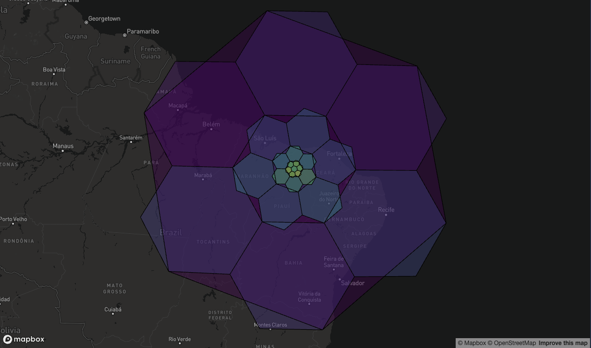
And if we continue to plot finer and finer resolution cells (all of which are children of the parent cell) we can start to see the rotation effect when changing resolution.
As you go from an odd-to-even resolution, the hexagons are rotated by ~19.1 degrees. Then as you go from even-to-odd, they are rotated back again.
So all the even-resolution cells are at the same orientation as each other, and similarly all the odd-resolution cells are at the same orientations as each other.
cells <- c('8081fffffffffff')

## Children and resolutions 1:4
children_cells <- unlist(h3r::cellToChildren(cells, 1L))
children_cells_res2 <- unlist(h3r::cellToChildren(children_cells[1], 2L))
children_cells_res3 <- unlist(h3r::cellToChildren(children_cells_res2[1], 3L))
children_cells_res4 <- unlist(h3r::cellToChildren(children_cells_res3[1], 4L))
mapdeck(
  libraries = "h3"
  , location = rev(as.numeric(cellToLatLng(cells)))
  , zoom = 3
  , style = mapdeck_style("dark")
  )  %>%
  add_h3(
    data = data.frame(
      x = c(cells, children_cells, children_cells_res2, children_cells_res3, children_cells_res4)
      )
    , hexagon = "x"
    , fill_colour = "x"
    , fill_opacity = 0.4
    , tooltip = "x"
    , stroke_colour = "#000000"
    , stroke_width = 5000
    , update_view = TRUE
  )
Cells and Coordinates
For this section we’ll be using the stations data from
the h3r package
##   stop_id    stop_name       lat      lon
## 1   15351      Sunbury -37.57909 144.7273
## 2   15353 Diggers Rest -37.62702 144.7199
## 3   19827  Stony Point -38.37423 145.2218
## 4   19828   Crib Point -38.36612 145.2040
## 5   19829     Morradoo -38.35403 145.1896
## 6   19830      Bittern -38.33739 145.1780
You can convert these coordinates to their containing cells…
df_stations$cell <- h3r::latLngToCell(
  lat = df_stations$lat
  , lng = df_stations$lon
  , resolution = 8
  )
head(df_stations)
## stop_id stop_name lat lon cell
## 1 15351 Sunbury -37.57909 144.7273 88be637a09fffff
## 2 15353 Diggers Rest -37.62702 144.7199 88be634497fffff
## 3 19827 Stony Point -38.37423 145.2218 88be606e81fffff
## 4 19828 Crib Point -38.36612 145.2040 88be606e95fffff
## 5 19829 Morradoo -38.35403 145.1896 88be606eb3fffff
## 6 19830 Bittern -38.33739 145.1780 88be606cdbfffff… but you can’t get the coordinates back again. You can only get the center coordinates for each cell.
Notice here how the returned coords are different to the
original coordinates
coords <- h3r::cellToLatLng(df_stations$cell)

cbind( head(coords), head(df_stations) )
## lat lng stop_id stop_name lat lon cell
## 1 -37.58134 144.7259 15351 Sunbury -37.57909 144.7273 88be637a09fffff
## 2 -37.62727 144.7150 15353 Diggers Rest -37.62702 144.7199 88be634497fffff
## 3 -38.37178 145.2217 19827 Stony Point -38.37423 145.2218 88be606e81fffff
## 4 -38.36837 145.1992 19828 Crib Point -38.36612 145.2040 88be606e95fffff
## 5 -38.35136 145.1916 19829 Morradoo -38.35403 145.1896 88be606eb3fffff
## 6 -38.34114 145.1766 19830 Bittern -38.33739 145.1780 88be606cdbfffff
# Notice how they are different to head(stations)Boundaries
If you want the cell as a spatial polygon you can get their
boundaries as coordinates, and convert to an sf object, as
in this example
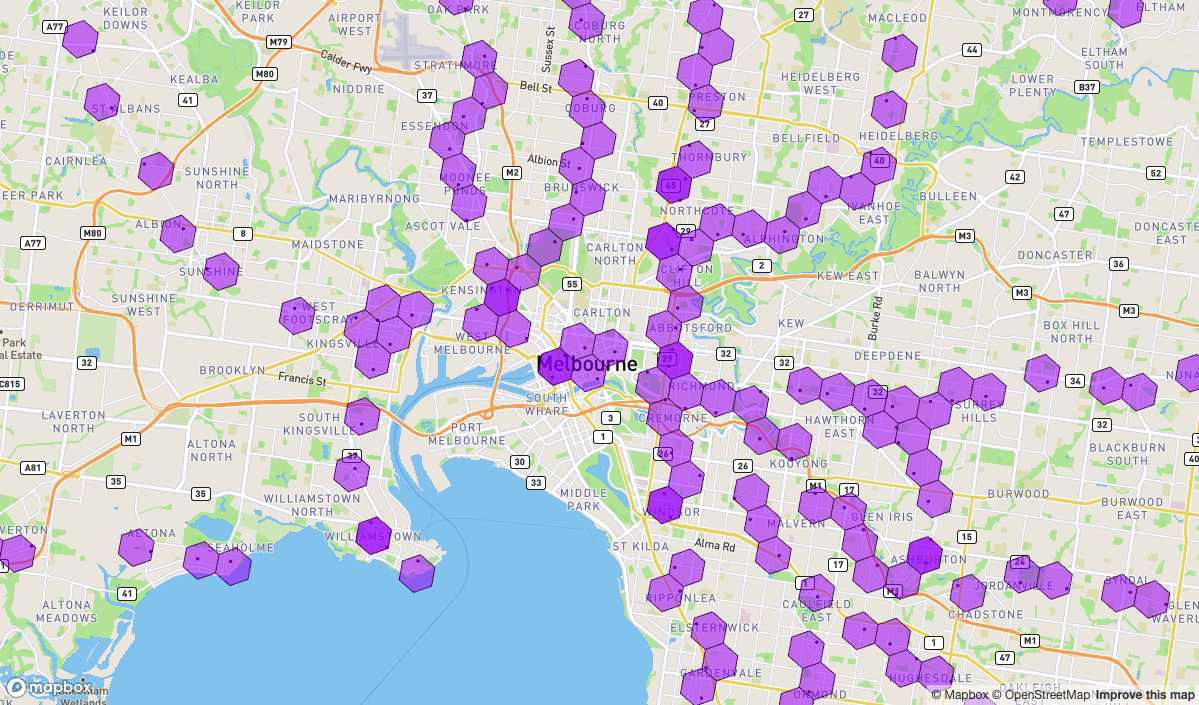
boundaries <- h3r::cellToBoundary(df_stations$cell)

## The `cellToBoundary` function returns a named list. Each element is named
## with the cell name, and the coordinatres are the vertieces of the hexagons.
##
## However, some stations are in the same cell
## so Replace the cell name with the stop name

names(boundaries) <- df_stations$stop_name

boundaries <- do.call(rbind, boundaries)
boundaries$id <- gsub("\\.[0-9]","",rownames(boundaries))

## Make a polygon
sf_boundaries <- sfheaders::sf_polygon(
  boundaries
  , x = "lng"
  , y = "lat"
  , polygon_id = "id"
  )
Notice in the map how some stations share the same cell (at resolution 8)
mapdeck(
  location = c(144.967590, -37.810935)
  , zoom = 11
  ) %>%
  add_scatterplot(
    data = df_stations
    , update_view = FALSE
    , radius = 50
  ) %>%
  add_polygon(
    sf_boundaries
    , fill_colour = '#9f19ff88'
    , stroke_width = 25
    , update_view = FALSE
  )
References
- H3: Tiling the Earth with Hexagons Youtube - Uber Engineering
- Tables of Cell Statistics Across Resolutions h3Geo.org