Simple simulation example • collision

library(collision)
library(Distance) # for distance modelling
#> Loading required package: mrds
#> This is mrds 3.0.1
#> Built: R 4.6.0; ; 2026-04-24 22:38:47 UTC; unix
#> 
#> Attaching package: 'Distance'
#> The following object is masked from 'package:mrds':
#> 
#>     create.bins
library(mc2d)  # for the PERT distribution
#> Loading required package: mvtnorm
#> 
#> Attaching package: 'mc2d'
#> The following objects are masked from 'package:base':
#> 
#>     pmax, pmin
library(ggplot2)
library(data.table) # for easy summarising and joins
#> 
#> Attaching package: 'data.table'
#> The following object is masked from 'package:base':
#> 
#>     %notin%

Stochastic Example

This is a good example to start with stochastic simulation. It models a (fictional) site with four proposed turbines, of two different models, and a (fictional) point count survey of a raptor species.

For this example we assume flight density is constant across the site.

We are going to calculate a simple stochastic model output here.

In the examples below we are just outlining how to use the model but there’s a lot of analysis required beforehand to fit a distance curve and extract the effective detection radius, analyse flight heights, and understand the spatial and temporal variability in the flight patterns. Please refer to other vignettes for more information.

The inner functions of the package are designed to take single value inputs. The input functions define_bird and define_turbine can define single or stochastic inputs. So we need to:

Define stochastic rules for inputs
- bird(s): define_bird()
- turbine(s): define_turbine()
- proportion of flights at and below rotor swept height
- effective detection radius (EDR): obtained from distance modelling (Buckland et al. 2001)
- encounter rate: encounter_rate()
Sample from the input distributions into the collision calculations to determine the distribution of possible collision outcomes.

This allows the simulation to more accurately reflect the uncertainty due to both natural variance (e.g. bird wingspan) and measurement uncertainty (e.g. estimated flight heights).

Define inputs

Turbine model

Step one is to set up a turbine - here’s some examples of two generic turbines, set up using the define_turbine function. These parameters can be defined as probability distributions or as single numbers.


turbine_model1 <- define_turbine(
  model_id = "Turbine 180",
  blade_length = 88,
  blade_thickness_narrow = 0.5,
  blade_thickness_wide = 3,
  d_base = 8.7,
  d_rotormin = 6.57,
  d_top = 3.5,
  hh = 149,
  max_chord = 5,
  min_chord = 2,
  max_nac_h = 3,
  max_nac_l = 20,
  max_width_nacelle = 3,
  rpm = set_random("rnorm", mean = 6.5, sd = 2),
  rotor_diam = 180,
  tilt_deg = 6,
  prop_operational = 0.98
)

turbine_model2 <- define_turbine(
  model_id = "Turbine 150",
  blade_length = 73.7,
  blade_thickness_narrow = 0.4,
  blade_thickness_wide = 3,
  d_base = 7,
  d_rotormin = 5.6,
  d_top = 3,
  hh = 112,
  max_chord = 4.2,
  min_chord = 1.5,
  max_nac_h = 3,
  max_nac_l = 13,
  max_width_nacelle = 3,
  rpm = set_random("rnorm", mean = 9.1, sd = 2),
  rotor_diam = 150,
  tilt_deg = 6,
  prop_operational = 0.98
)

Bird species

We make a ‘bird’ object - a list of key parameters. These parameters can be defined as probability distributions or as single numbers.


wte <- define_bird(
  species = "Wedge-tailed Eagle",
  bird_length = set_random("rnorm", mean = 0.945, sd = 0.2) ,
  bird_speed = set_random("rnorm", mean = 17, sd = 3),
  prop_day = set_random("runif", min = 0.48, max = 0.52),
  prop_year = 1,
  avoidance_dynamic = set_random("rpert",
                                 min = 0.88, max = 0.95, 
                                 mode = 0.92, shape = 4),
  avoidance_static = 0.9999
)

Note: the Beta PERT distribution (rpert) is a good distribution to use if you only have the mode (or mean) and the minimum and maximum parameters for a species (eg. mean body length = 0.95m, range: 0.6-1.2m). See the Choosing Distributions¹ for information on how to fit the distributions.

Define a Set of Turbines

The basic template for the model outputs is a data.frame of turbine inputs. These can be read in from a csv, or you can set them up with a few basic pieces of information and the turbine definition above.

For each turbine we need a turbine ID, and a location. Location can be NA if you are not including any spatial modelling.

df_turbines <- data.frame(
  turbine_id = c("T01", "T02", "T03", "T04"),
  model = rep(c("Turbine 180", "Turbine 150"), each = 2),
  lat = c(-32.505, -32.521, -32.523, -32.516),
  lon = c(143.441, 143.442, 143.425, 143.457)
)

Survey data

Now we need to determine the input values from the observations. In order to determine the error on the estimate of the parameter we use the bootstrap method to repeatedly resample the distribution. This is just an example of how you can obtain the distribution, it is up to the analyst to determine how best to model these parameters.

The package observations dataset:

summary(df_obs)
#>     distance           size            type         height      
#>  Min.   :  71.0   Min.   :1.0   Length   :120   Min.   :  43.0  
#>  1st Qu.: 534.8   1st Qu.:1.0   N.unique :  1   1st Qu.: 328.0  
#>  Median : 763.0   Median :1.0   N.blank  :  0   Median : 662.0  
#>  Mean   : 805.4   Mean   :1.3   Min.nchar:  6   Mean   : 730.5  
#>  3rd Qu.:1027.0   3rd Qu.:2.0   Max.nchar:  6   3rd Qu.: 986.2  
#>  Max.   :1878.0   Max.   :2.0                   Max.   :2469.0  
#>    survey_id          object      
#>  Min.   :  1.00   Min.   :  1.00  
#>  1st Qu.: 29.75   1st Qu.: 30.75  
#>  Median : 60.00   Median : 60.50  
#>  Mean   : 53.91   Mean   : 60.50  
#>  3rd Qu.: 78.00   3rd Qu.: 90.25  
#>  Max.   :100.00   Max.   :120.00
# converting to data.table for ease of joining and summarising
dt_obs <- setDT(copy(df_obs))

is a dataset of 120 observations from 100 point count surveys, including the count (size) of raptors and associated distance at first observation (distance).

And the package survey dataset:

summary(df_survey)
#>    survey_id      survey_duration    survey_type 
#>  Min.   :  1.00   Min.   :45      Length   :100  
#>  1st Qu.: 25.75   1st Qu.:45      N.unique :  1  
#>  Median : 50.50   Median :45      N.blank  :  0  
#>  Mean   : 50.50   Mean   :45      Min.nchar:  5  
#>  3rd Qu.: 75.25   3rd Qu.:45      Max.nchar:  5  
#>  Max.   :100.00   Max.   :45

dt_survey <- setDT(copy(df_survey))

is a dataset of the metadata for the 100 point count surveys, including the duration of each survey.

It’s very important that the field data include any surveys with no sightings as well as positive detections.

Between the two of them these tables must include:

Distance to the bird at first sighting in metres. If transect sampling, this is usually the perpendicular (right-angle) distance from the transect line.
Duration of the surveys in minutes
Count of individuals in each survey (size)

Effective Detection Radius

For this example, we assume you have done the required distance correction and have arrived at a distance model.

summary(ds_raptor)
#> 
#> Summary for distance analysis 
#> Number of observations :  120 
#> Distance range         :  0  -  2334 
#> 
#> Model       : Half-normal key function with cosine adjustment terms of order 2,3 
#> 
#> Strict monotonicity constraints were enforced.
#> AIC         :  1812.536 
#> Optimisation:  mrds (slsqp) 
#> 
#> Detection function parameters
#> Scale coefficient(s):  
#>             estimate         se
#> (Intercept) 6.822439 0.08498135
#> 
#> Adjustment term coefficient(s):  
#>                 estimate        se
#> cos, order 2 -0.33444481 0.1543828
#> cos, order 3  0.09652554 0.1490168
#> 
#>                        Estimate        SE        CV
#> Average p             0.6314592  0.141781 0.2245292
#> N in covered region 190.0360410 43.949117 0.2312673

Rather than extracting the EDR from this model (which would give us a single value) we bootstrap the distance model and the EDR to obtain the standard deviation on the estimate of the EDR.

## Define bootstrap-able function
edr_fun <- function(dt_survey = dt_survey,
                    i = nrow(dt_survey),
                    dt_obs = dt_obs){
  
  dt_boot_i <- dt_survey[i][order(survey_id)]
  dt_obs_i <- dt_obs[dt_boot_i[, .(survey_id)]
                     , on = .(survey_id)
                     , nomatch = 0]
  
  ds_CI <- tryCatch(
    ds(data = dt_obs_i[, -c("object")],
       formula = ~ 1,
       key = "hn",
       dht_group = TRUE) # same arguments used to fit the original distance model (ds_raptor)
    , error = function(e) {
      print(e)
      NULL
    }
  )

  if (is.null(ds_CI)) return(NA)
  edr_boot <- edr_from_distmodel(ds_CI)
  return(edr_boot)
}

ds_boot <- boot::boot(data = dt_survey
                , statistic = edr_fun,
                , sim = "ordinary"
                , stype = "i"
                , R = 150
                , dt_obs = dt_obs
)
# bootstraps need to be checked for convergence to make sure you've done enough replicates
# which is not done in this example

## Define EDR
edr <- set_random("rnorm", # normally distributed per CLT
                  mean = ds_boot$t0,
                  sd = sd(ds_boot$t, na.rm = TRUE)
                  )

## visual check of distribution
EDR_hist <- sapply(1:1000, FUN = function(i) collision::sample_input(edr) )
hist(EDR_hist)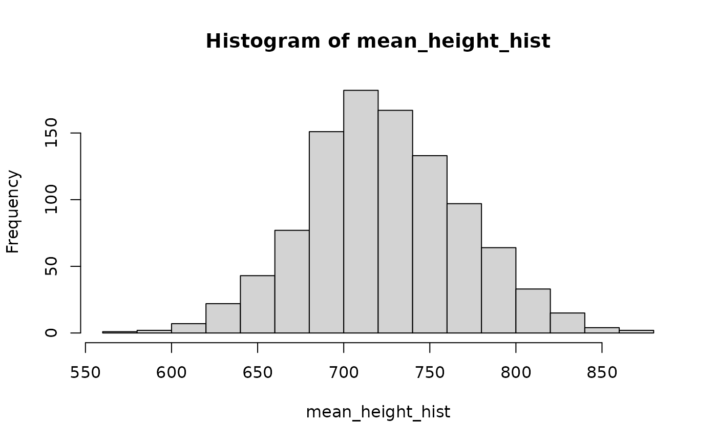

Flight heights

In order to determine the flight flux we need an effective detection height, but unlike with the EDR we can’t fit a distance model to the heights because distance modelling relies on the assumption that the birds are uniformly distributed at all distances, which we know is not the case in vertical space (i.e. the density of flights tends to drop off with increasing height). The simplest way to avoid biasing the estimate by artificially inflating or deflating the flux through the turbine is to desktop truncate the observations to the maximum tip height of the turbine and use that as the effective detection height (all the observations can still be used to fit the observer’s detection function since it is just used for the horizontal distance correction). Other methods for estimating an effective detection height can be used, but this method is the most straightforward and will work well in almost all cases. Truncating the the maximum turbine height also means that the proportion of flights at rotor swept height (prop_at_height) and below rotor swept height (prop_below_height) sum to 1.

The proportion of flights at and below rotor swept height account for the amount of flights at risk of being struck by the blades of the turbine. We only need to calculate a distribution for prop_below_height since prop_at_height = 1 - prop_below_height.

min_rsh1 <- turbine_model1$hh - turbine_model1$rotor_diam * 0.5
max_rsh1 <- turbine_model1$hh + turbine_model1$rotor_diam * 0.5

min_rsh2 <- turbine_model2$hh - turbine_model2$rotor_diam * 0.5
max_rsh2 <- turbine_model2$hh + turbine_model2$rotor_diam * 0.5

## calculate ecdf
# Note - this is a simple example; it's up to the analyst how best to fit the height distribution

prop_below <- function(dt_survey = dt_survey,
                       i = seq_len(nrow(dt_survey)),
                       dt_obs = dt_obs, # filter by max_rsh
                       h = max_rsh){
  
  dt_boot_i <- dt_survey[, .(survey_id = unique(survey_id))][i]
  dt_obs_i <- dt_obs[dt_boot_i, on = .(survey_id), nomatch = 0]
  
  cdf_dat <- ecdf(dt_obs_i$height)
  
  return(cdf_dat(h))
}

# turbine model 1
## bootstrap prop below min RSH
hmin_boot1 <- boot::boot(
  data = dt_survey,
  statistic = prop_below, stype = "i",
  R = 900,
  h = min_rsh1,
  dt_obs = dt_obs[height <= max_rsh1]
)

prop_below_height1 <- set_random("rnorm", mean = hmin_boot1$t0, sd = sd(hmin_boot1$t))
# you may need to use a bounded distribution if the proportion is near 0 or 1

# turbine model 2
## bootstrap prop below min RSH
hmin_boot2 <- boot::boot(
  data = dt_survey,
  statistic = prop_below, stype = "i",
  R = 900,
  h = min_rsh2,
  dt_obs = dt_obs[height <= max_rsh2]
)

prop_below_height2 <- set_random("rnorm", mean = hmin_boot2$t0, sd = sd(hmin_boot2$t))

Encounter Rate

This is where we determine the average encounter rate per unit time of survey. That is the average number of individuals observed in each minute of survey (or whatever unit of time you wish to use). This is basically just $\frac{total\ individuals\ observed}{total\ survey\ time}$ , however the function also allows for weighting surveys to account for stratification and can apply the Wilson correction (Wilson 1927) if there were no observations.

As discussed above, we are desktop truncating to the maximum rotor swept height of the turbine, so this encounter rate will be the encounter of birds at risk height.

This function takes as input a df_obs_summary data.frame. This object has one row per survey and must contain a column named survey_duration and a column named size which is the total number of individuals observed in each survey (not observation). Optionally, it can contain a column named survey_weight which has the associated relative weights of each survey (to avoid artificially inflating or deflating the encounter rate sum(survey_weight) must equal the number of surveys).

First let’s make that table (using data.table):

# turbine model 1
dt_obs_survey1 <- dt_obs[height <= max_rsh1, .("size" = sum(size)), survey_id][dt_survey,
                                                            on = "survey_id"]
# need sum(size) because we want one row per survey (not observation)
setnafill(dt_obs_survey1, cols = c("size"), fill = 0) # set size to 0 for surveys with no observations

# turbine model 2
dt_obs_survey2 <- dt_obs[height <= max_rsh2, .("size" = sum(size)), survey_id][dt_survey,
                                                            on = "survey_id"]
setnafill(dt_obs_survey2, cols = c("size"), fill = 0)

Now we can use this table in encounter_rate():


er_fun <- function(dat, i){
  return(encounter_rate(df_obs_summary = dat[i]))
}

# turbine model 1
er_boot1 <- boot::boot(data = dt_obs_survey1
                , statistic = er_fun,
                , sim = "ordinary"
                , stype = "i"
                , R = 200
)


## Define Encounter rate
flights_per_min1 <- set_random("rnorm",
                               mean = er_boot1$t0,
                               sd = sd(er_boot1$t, na.rm = TRUE)
                               )

## take a look

encounter_rate_hist1 <- sapply(1:1000, FUN = function(i) collision::sample_input(flights_per_min1) )
hist(encounter_rate_hist1)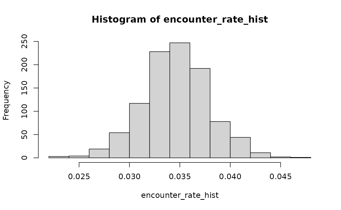


# turbine model 2
er_boot2 <- boot::boot(data = dt_obs_survey2
                , statistic = er_fun,
                , sim = "ordinary"
                , stype = "i"
                , R = 200
)


## Define Encounter rate
flights_per_min2 <- set_random("rnorm",
                               mean = er_boot2$t0,
                               sd = sd(er_boot2$t, na.rm = TRUE)
                               )

## take a look

encounter_rate_hist2 <- sapply(1:1000, FUN = function(i) collision::sample_input(flights_per_min2) )
hist(encounter_rate_hist2)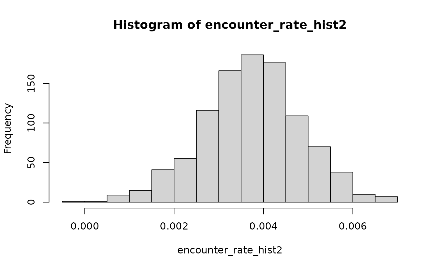

Run the simulation

Here we set up a loop to run the simulation. Note that each iteration of the loop is independent to others, meaning that you can wrap the loop inside methods to run the iterations in parallel to save time if you wish.

Step 0 - Set up simulation parameters
Step 1 - Sample inputs for bird, turbine, prop at height, prop below height, effective detection radius (EDR) and encounter rate.
Step 1.5 (optional) - Calculate the cluster_correction or any spatial flight corrections. The cluster correction is only needed if the distance between turbines $\leq$ EDR.
Step 2 - Calculate turbine_flights_year() with sampled values - calculate flights through turbine per year
Step 3 - Run prob_collision_static() and prob_collision_dynamic() - calculate $P(C|I)$ for one interaction
Step 4 - Run n_collisions() - calculate number of collisions a year

For a breakdown of each step see the deterministic example.

## inputs needed:
## seed for reproducibility
## iterations - how many runs
## df_turbines  - class `data.frame`
## wte - class `birdInput`
## v90_single - class `turbineInput`
## prop_at_height - class `randomInput`
## prop_below_height - class `randomInput`
## edr - class `randomInput`
## encounter rate - class `randomInput`
## mean height - class `randomInput`


set.seed(1234)
iterations <- 1000

lst_results <- lapply(1:iterations, function(i) {
  df_turbines_results <- df_turbines

  # Step 1 - Sample inputs for bird, turbine, prop at height and prop below height
  bird_i <- sample_input(wte)
  edr_i <- sample_input(edr)
  
  turbines1_i <- sample_input(turbine_model1)
  prop_below_height1_i <- max( sample_input(prop_below_height1), 0)
  prop_at_height1_i <- 1-prop_below_height1_i
  
  er1_i <- sample_input(flights_per_min1)
  
  turbines2_i <- sample_input(turbine_model2)
  prop_below_height2_i <- sample_input(prop_below_height2)
  prop_at_height2_i <- 1-prop_below_height2_i
  er2_i <- sample_input(flights_per_min2)
  
  # Step 1.5 calculate the cluster correction
  
  df_turbines_results$cluster_corr <- cluster_correction_a(
    eff_detection_width = 2*edr_i,
    df_turbines = df_turbines_results
  )
  
  # Step 2 calculate flux through turbine per year
  df_turbines_results[df_turbines_results$model == "Turbine 180",
                      "flight_turbine_year"] <- turbine_flights_year(
    survey_type = c("point"),
    encounter_rate = er1_i,
    eff_detection_width = 2*edr_i,
    eff_detection_height = max_rsh1,
    spatial_correction = df_turbines_results[df_turbines_results$model == "Turbine 180",
                      "cluster_corr"],
    rotor_diameter = turbines1_i$rotor_diam,
    hub_height = turbines1_i$hh,
    prop_day = bird_i$prop_day,
    prop_year = bird_i$prop_year
  )
  
  df_turbines_results[df_turbines_results$model == "Turbine 150",
                      "flight_turbine_year"] <- turbine_flights_year(
    survey_type = c("point"),
    encounter_rate = er2_i,
    eff_detection_width = 2*edr_i,
    eff_detection_height = max_rsh2,
    spatial_correction = df_turbines_results[df_turbines_results$model == "Turbine 150",
                      "cluster_corr"],
    rotor_diameter = turbines2_i$rotor_diam,
    hub_height = turbines2_i$hh,
    prop_day = bird_i$prop_day,
    prop_year = bird_i$prop_year
  )

  # Step 3 - Run `p_collisions()` - calculate $P(C|I)$ for one interaction
  df_turbines_results[df_turbines_results$model == "Turbine 180",
                      "p_coll_static"] <- prob_collision_static(
    d_base = turbines1_i$d_base,
    d_rotormin = turbines1_i$d_rotormin,
    d_top = turbines1_i$d_top,
    hh = turbines1_i$hh,
    blade_length = turbines1_i$blade_length,
    max_nac_h = turbines1_i$max_nac_h,
    max_nac_l = turbines1_i$max_nac_l,
    max_width_nacelle = turbines1_i$max_width_nacelle,
    rotor_diam = turbines1_i$rotor_diam,
    tilt_deg = turbines1_i$tilt_deg,
    max_chord = turbines1_i$max_chord,
    min_chord = turbines1_i$min_chord,
    blade_thickness_wide = turbines1_i$blade_thickness_wide,
    blade_thickness_narrow = turbines1_i$blade_thickness_narrow,
    prop_at_height = prop_at_height1_i,
    prop_below_height = prop_below_height1_i
  )
  
  df_turbines_results[df_turbines_results$model == "Turbine 150",
                      "p_coll_static"] <- prob_collision_static(
    d_base = turbines2_i$d_base,
    d_rotormin = turbines2_i$d_rotormin,
    d_top = turbines2_i$d_top,
    hh = turbines2_i$hh,
    blade_length = turbines2_i$blade_length,
    max_nac_h = turbines2_i$max_nac_h,
    max_nac_l = turbines2_i$max_nac_l,
    max_width_nacelle = turbines2_i$max_width_nacelle,
    rotor_diam = turbines2_i$rotor_diam,
    tilt_deg = turbines2_i$tilt_deg,
    max_chord = turbines2_i$max_chord,
    min_chord = turbines2_i$min_chord,
    blade_thickness_wide = turbines2_i$blade_thickness_wide,
    blade_thickness_narrow = turbines2_i$blade_thickness_narrow,
    prop_at_height = prop_at_height2_i,
    prop_below_height = prop_below_height2_i
  )

  df_turbines_results[df_turbines_results$model == "Turbine 180",
                      "p_coll_dyn"] <- prob_collision_dynamic(
    rpm = turbines1_i$rpm, # s_rot,
    blade_length = turbines1_i$blade_length,
    max_width_nacelle = turbines1_i$max_width_nacelle,
    rotor_diam = turbines1_i$rotor_diam,
    blade_thickness_wide = turbines1_i$blade_thickness_wide,
    blade_thickness_narrow = turbines1_i$blade_thickness_narrow,
    hh = turbines1_i$hh,
    bird_length = bird_i$bird_length,
    bird_speed = bird_i$bird_speed,
    prop_at_height = prop_at_height1_i,
    prop_below_height = prop_below_height1_i,
    prop_operational = turbines1_i$prop_operational
  )
  
  df_turbines_results[df_turbines_results$model == "Turbine 150",
                      "p_coll_dyn"] <- prob_collision_dynamic(
    rpm = turbines2_i$rpm, # s_rot,
    blade_length = turbines2_i$blade_length,
    max_width_nacelle = turbines2_i$max_width_nacelle,
    rotor_diam = turbines2_i$rotor_diam,
    blade_thickness_wide = turbines2_i$blade_thickness_wide,
    blade_thickness_narrow = turbines2_i$blade_thickness_narrow,
    hh = turbines2_i$hh,
    bird_length = bird_i$bird_length,
    bird_speed = bird_i$bird_speed,
    prop_at_height = prop_at_height2_i,
    prop_below_height = prop_below_height2_i,
    prop_operational = turbines2_i$prop_operational
  )


  # Step 4 - Run `n_collisions()` - calculate number of collisions a year
  df_turbines_results$n_collision <- n_collision(
    avoidance_rate_static = bird_i$avoidance_static,
    avoidance_rate_dynamic = bird_i$avoidance_dynamic,
    n_flights = df_turbines_results$flight_turbine_year,
    p_coll_static = df_turbines_results$p_coll_static,
    p_coll_dynamic = df_turbines_results$p_coll_dyn
  )

  ## for reporting - optional
  df_turbines_results$iteration <- i

  return(df_turbines_results)
})

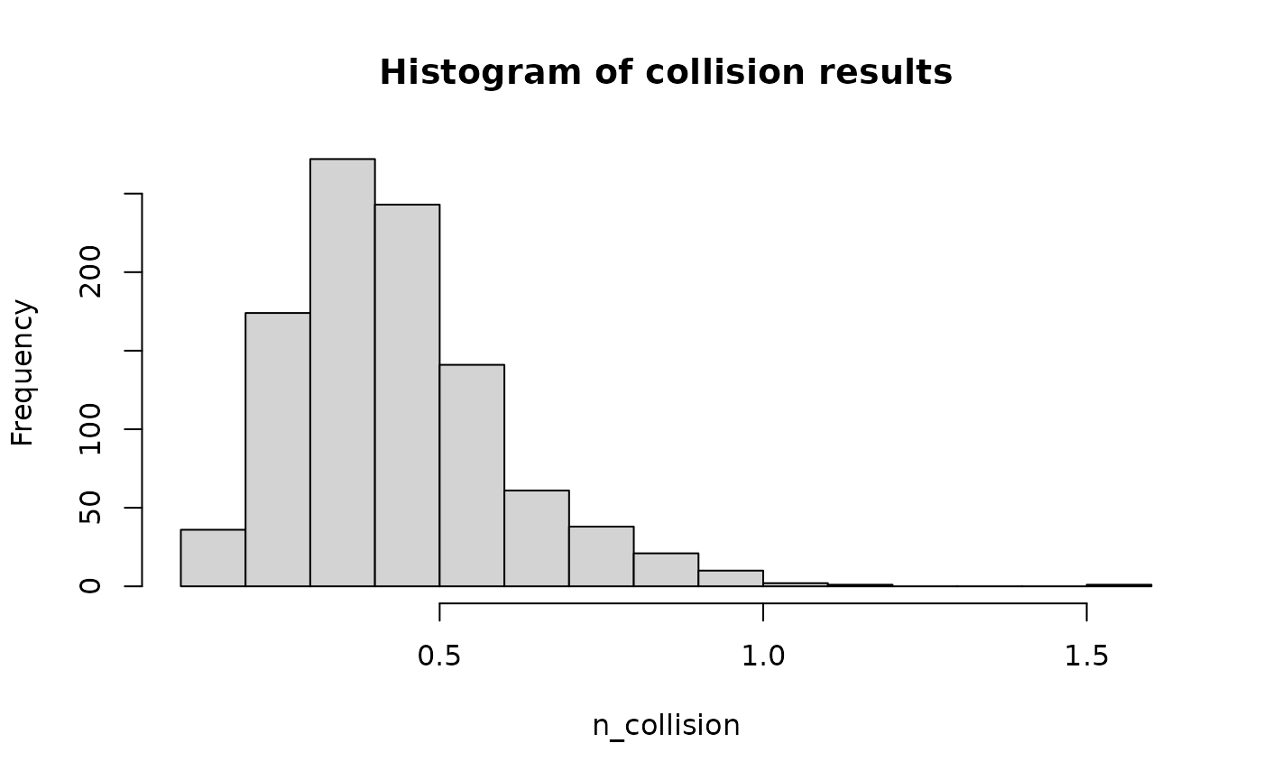
Now we have the output of each simulation. We can use them to plot out the histogram of collision results. This shows the distribution of the long-term average annual collision rate for the wind farm.

lapply(lst_results, function(x) {
  sum(x$n_collision)
}) |>
  unlist() |>
  hist(x = _, xlab = "n_collision", main = "Histogram of collision results")

References

Buckland, S., D. Anderson, K. Burnham, Jeffrey Laake, David Borchers, and Len Thomas. 2001. Introduction to Distance Sampling: Estimating Abundance of Biological Populations. Xv. Oxford University Press. https://doi.org/10.1093/oso/9780198506492.001.0001.

Wilson, Edwin B. 1927. “Probable Inference, the Law of Succession, and Statistical Inference.” Journal of the American Statistical Association 22 (158): 209–12. https://doi.org/10.1080/01621459.1927.10502953.