Deterministic example

library(knitr)
library(collision)
library(ggplot2)

# for easy summarising and joins
library(data.table)

# for distance modelling
library(Distance)
#> Loading required package: mrds
#> This is mrds 3.0.1
#> Built: R 4.5.0; ; 2025-07-06 04:17:12 UTC; unix
#> 
#> Attaching package: 'Distance'
#> The following object is masked from 'package:mrds':
#> 
#>     create.bins

This is a good example to start with. It models a (fictional) site with 2 proposed turbines, all of the same model, and a (fictional) point count survey of Wedge-tailed Eagle. For this example we assume flight density is constant across the site.

We are going to calculate a simple deterministic model output here. For a stochastic output see the other examples.

Setup inputs

Define turbine model

Step one is to set up a turbine - here’s an example based on a Vestas 90, set up using the define_turbine function:

v90_single <- define_turbine(
  model_id = "Vesta V90",
  blade_length = 44,
  blade_thickness_narrow = 0.07,
  blade_thickness_wide = 2.6,
  d_base = 4.15,
  d_rotormin = 3.55,
  d_top = 2.55,
  hh = 65,
  max_chord = 3.51,
  min_chord = 0.39,
  max_nac_h = 4.05,
  max_nac_l = 13.25,
  max_width_nacelle = 3.6,
  rpm = 16.1,
  rotor_diam = NULL,
  tilt_deg = 6,
  prop_operational = 0.98
)

Define bird

Now we need a bird (see define_bird)

wte <- define_bird(
  species = "Wedge-tailed Eagle",
  bird_length = 0.945,
  bird_speed = 17,
  prop_day = 0.5,
  prop_year = 1,
  avoidance_dynamic = 0.90,
  avoidance_static = 0.9999
)

Define a set of turbines

The basic template for the model outputs is a data.frame of turbine inputs. These can be read in from a csv, or you can set them up with a few basic pieces of information and the turbine definition above.

For each turbine we need a turbine ID, and a location. Location can be NA if you are not including any spatial modelling.

make_turbine_set creates the data.frame of turbine inputs, sampled (if needed) and ready for analysis


df_turbines <- data.frame(
  turbine_id = c("T01", "T02"),
  lat = c(-32.512, -32.521),
  lon = c(143.441, 143.442)
)

Survey, observation and detection radius

Use the provided survey data to fit a (very simple) distance model. NOTE Please see Distance and the references therein for a complete primer on doing and interpreting Distance analysis.

The package observations dataset:

summary(df_obs)
#>     distance           size         type               height      
#>  Min.   :  71.0   Min.   :1.0   Length:120         Min.   :  43.0  
#>  1st Qu.: 534.8   1st Qu.:1.0   Class :character   1st Qu.: 328.0  
#>  Median : 763.0   Median :1.0   Mode  :character   Median : 662.0  
#>  Mean   : 805.4   Mean   :1.3                      Mean   : 730.5  
#>  3rd Qu.:1027.0   3rd Qu.:2.0                      3rd Qu.: 986.2  
#>  Max.   :1878.0   Max.   :2.0                      Max.   :2469.0  
#>    survey_id          object      
#>  Min.   :  1.00   Min.   :  1.00  
#>  1st Qu.: 29.75   1st Qu.: 30.75  
#>  Median : 60.00   Median : 60.50  
#>  Mean   : 53.91   Mean   : 60.50  
#>  3rd Qu.: 78.00   3rd Qu.: 90.25  
#>  Max.   :100.00   Max.   :120.00

is a dataset of 120 observations from 100 point count surveys, including the count (size) of raptors (and associated distance at first observation (distance)).

And the package survey dataset:

summary(df_survey)
#>    survey_id      survey_duration survey_type       
#>  Min.   :  1.00   Min.   :45      Length:100        
#>  1st Qu.: 25.75   1st Qu.:45      Class :character  
#>  Median : 50.50   Median :45      Mode  :character  
#>  Mean   : 50.50   Mean   :45                        
#>  3rd Qu.: 75.25   3rd Qu.:45                        
#>  Max.   :100.00   Max.   :45

is a dataset of the metadata for the 100 point count surveys, including the duration of each survey.

It’s very important that the field data include any surveys with no sightings as well as positive detections.

Between the two of them these tables must include:

Distance to the bird at first sighting in metres. If transect sampling, this is usually the perpendicular (right-angle) distance from the transect line.
Duration of the surveys in minutes
Count of individuals in each survey (size)

We fit a distance model and extract the effective detection radius (EDR). The effective detection radius is the radius of a circle, such that if 100% of flights were observed within this circle, the expected number of flights detected is the same as for the actual survey (which has decaying detectability with distance).

ds_model <- ds(
  data = df_obs,
  truncation = max(df_obs$distance, na.rm=TRUE),
  transect = "point",
  formula = ~1,
  key = "hr",
  dht_group = TRUE,
  nadj = 0
  )
#> Fitting hazard-rate key function
#> AIC= 1772.74
#> No survey area information supplied, only estimating detection function.

plot(ds_model, pdf=TRUE)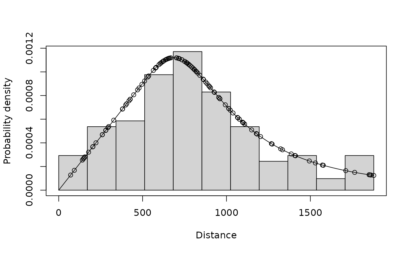


print(edr_from_distmodel(ds_model)) # in metres
#> [1] 1052.974
print(w_from_distmodel(ds_model)) # truncation distance / max distance in m
#> [1] 1878

Calculate proportion at height and below height

prop_at_height is either a single value or distribution information which represents the proportion of flights at rotor swept height while prop_below_height is the proportion of flights below rotor swept height.

A simple, single value example of this is given below


# rotor_diam / 2 is better than using blade length because it 
# includes the nacelle size 
min_rsh <- v90_single$hh - v90_single$rotor_diam * 0.5
max_rsh <- v90_single$hh + v90_single$rotor_diam * 0.5

## Review the heights
ggplot(data = as.data.frame(df_obs),
       aes(x = height, y = after_stat(density))) +
  geom_histogram() +
  geom_vline(xintercept = min_rsh, colour = "red") +
  geom_vline(xintercept = max_rsh, colour = "red")
#> `stat_bin()` using `bins = 30`. Pick better value `binwidth`.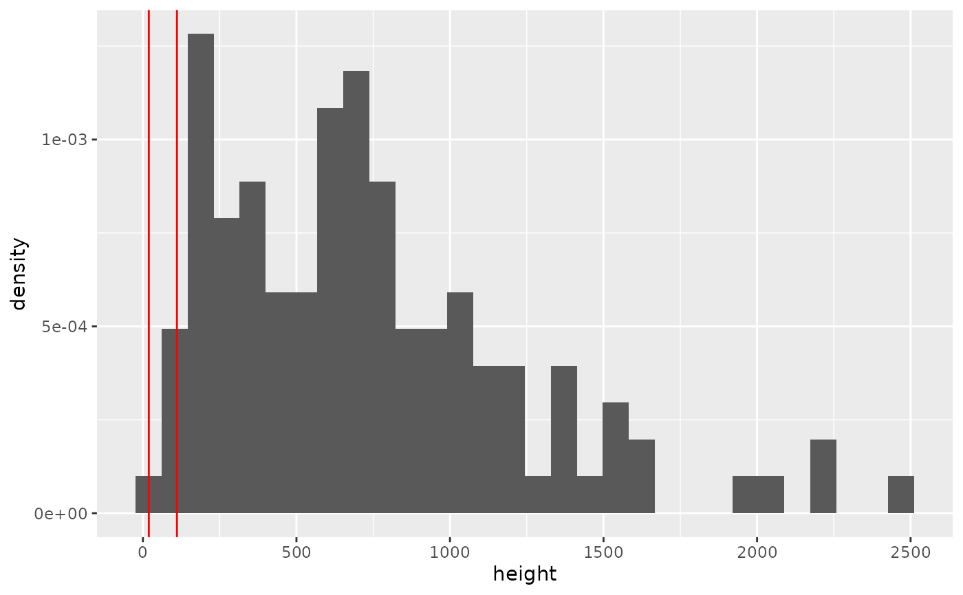



# calculate ecdf (empirical cumulative distribution function)
# Note - this is a simple example; it's up to the analyst how best to 
## fit the height distribution
cdf_height <- ecdf(df_obs$height)

prop_at_height <- cdf_height(round(max_rsh)) - cdf_height(round(min_rsh))
prop_below_height <- cdf_height(round(min_rsh))

Proportion at height: 0.0333333
Proportion below height: 0
Proportion above height: 0.9666667

Modelling

For a deterministic model, we need the following 4 steps:

Step 1 - Run encounter_rate() - calculate the uncorrected flights per survey minute.
Step 2 - Run obs_flux(), turbine_flux() and flux_per_year() - calculate flux through turbine per year. This can also be done in one step using turbine_flux_year().
Step 3 - Run prob_collision_static() and prob_collision_dynamic() - calculate $P(C|I)$ for one interaction
Step 4 - Run n_collisions() - calculate number of collisions a year

Step 1 - Encounter rate

This is where we determine the average encounter rate per unit time of survey. That is the average number of individuals observed in each minute of survey (or whatever unit of time you wish to use). This is basically just $\frac{total\ individuals\ observed}{total\ survey\ time}$ , however the function also allows for weighting surveys to account for stratification and can apply the Wilson correction (Wilson 1927) if there were no observations. The Wilson correction is an estimate of the encounter rate (mid-point of the 95% CI) that could result in zero observations.

This function takes as input a df_obs_summary data.frame. This object has one row per survey and must contain a column named survey_duration and a column named size which is the total number of individuals observed in each survey (not observation). Optionally, it can contain a column named survey_weight which has the associated relative weights of each survey (to avoid artificially inflating or deflating the encounter rate sum(survey_weight) must equal the number of surveys).

First let’s make that table (using data.table):

dt_obs <- copy(df_obs)
dt_survey <- copy(df_survey)

setDT(dt_obs)
setDT(dt_survey)

dt_obs_survey <- dt_obs[, .("size" = sum(size)), survey_id][dt_survey,
                                                            on = "survey_id"]
# need sum(size) because we want one row per survey (not observation)

Now we can use this table in encounter_rate():

flights_per_min <- encounter_rate(
  df_obs_summary = dt_obs_survey,
  wilson_correction = TRUE # Default
 )
#> Warning in encounter_rate(df_obs_summary = dt_obs_survey, wilson_correction =
#> TRUE): NA observations detected - NA observation size will be assumed to be 0

Any surveys with NA observations are assumed to have zero observations, which, if you left join to the survey table by survey_id, should be correct. The average number of movements observed per minute of survey is 0.0346667 flights per minute.

Step 2 - Flux through turbine

This is where we account for

The flight heights (mean_flight_height)
The observer’s detection model (eff_detection_width obtained using edr_dist_model())
The size of the turbine (contained in the object made using define_turbine())
The proportion of the day active (contained in the object made using define_bird())
The proportion of the year active (contained in the object made using define_bird())

We first calculate the observed flux through a vertical airspace. This is in flights per unit time per unit area, in this example the units are minutes and metres squared, respectively.

Second we apply this to the “turbine plane” (a rectangular “doorway” defined by the rotor diameter and maximum rotor swept height) using turbine_flights() to obtain the flights through the turbine plane per minute.


# flights / m / min
obs_flux_min <- obs_flux(
  encounter_rate = flights_per_min, # numeric per min
  eff_detection_width = 2.0*edr_from_distmodel(ds_model),
  mean_flight_height = mean(df_obs$height*df_obs$size) # weighted by individuals
)

#flights through turbine / min

turbine_flights_min <- turbine_flights(
  obs_flux = obs_flux_min,
  rotor_diameter  = v90_single$rotor_diam,
  hub_height = v90_single$hh
)

The observed flight flux is 8.7283936^{-9} flights per square metre per minute. Scaling up to the turbine this corresponds to 8.8586911^{-5} flights through the turbine area per minute.

Here we correct it for daily and monthly variability. This can be done by hand but the package includes a helper function which can scale to a year.

turbine_flight_year <- flights_per_year(
  flights_per_time = turbine_flights_min,
  time_units = "min",
  prop_day = wte$prop_day, # diurnal
  prop_year = wte$prop_year # present all year
)

The units for turbine_flight_year is flights / year (per turbine).
We expect 23.2965859 flights through the turbine area each year.

Step 3 - Probability of collision given interaction

Our approach considers both the static ( $P(C)_{s}$ ) and dynamic components ( $P(C)_{dyn}$ )

Without avoidance, and isolated from the overall collision rate calculation, the total probability of collision, given interaction is the

$P(C|I) = P(C|I)_{static} + P(C|I)_{dynamic}$

because the two options are mutually exclusive.

Let’s calculate the collision probability for a Wedge-tailed Eagle and the V90 turbine model.

df_turbines$p_coll_static <- prob_collision_static(
  d_base = v90_single$d_base,
  d_rotormin = v90_single$d_rotormin,
  d_top = v90_single$d_top,
  hh = v90_single$hh,
  blade_length = v90_single$blade_length,
  max_nac_h = v90_single$max_nac_h,
  max_nac_l = v90_single$max_nac_l,
  max_width_nacelle = v90_single$max_width_nacelle,
  rotor_diam = v90_single$rotor_diam,
  tilt_deg = v90_single$tilt_deg,
  max_chord = v90_single$max_chord,
  min_chord = v90_single$min_chord,
  blade_thickness_wide = v90_single$blade_thickness_wide,
  blade_thickness_narrow = v90_single$blade_thickness_narrow,
  prop_at_height = prop_at_height,
  prop_below_height = prop_below_height
)

df_turbines$p_coll_dyn <- prob_collision_dynamic(
  rpm = v90_single$rpm, 
  blade_length = v90_single$blade_length,
  max_width_nacelle = v90_single$max_width_nacelle,
  rotor_diam = v90_single$rotor_diam,
  blade_thickness_wide = v90_single$blade_thickness_wide,
  blade_thickness_narrow = v90_single$blade_thickness_narrow,
  hh = v90_single$hh,
  bird_length = wte$bird_length,
  bird_speed = wte$bird_speed,
  prop_at_height = prop_at_height,
  prop_below_height = prop_below_height
)

Step 4 - Total annual collisions (with avoidance)

Now using the calculated yearly interactions (flights through the turbine area) and probability of collision given interaction as well as the expected avoidance rates, we can obtain an estimate of the total number of expected collision per year.



df_turbines$n_collision <- n_collision(
  avoidance_rate_static = wte$avoidance_static,
  avoidance_rate_dynamic = wte$avoidance_dynamic,
  n_flights = turbine_flight_year,
  p_coll_static = df_turbines$p_coll_static,
  p_coll_dynamic = df_turbines$p_coll_dyn
)

## For a final result, sum all turbines
sum(df_turbines$n_collision)
#> [1] 0.2689028

References

Buckland, S., D. Anderson, K. Burnham, Jeffrey Laake, David Borchers, and Len Thomas. 2001. Introduction to Distance Sampling: Estimating Abundance of Biological Populations. Vol. xv. Oxford University Press. https://doi.org/10.1093/oso/9780198506492.001.0001.

Wilson, Edwin B. 1927. “Probable Inference, the Law of Succession, and Statistical Inference.” Journal of the American Statistical Association 22 (158): 209–12. https://doi.org/10.1080/01621459.1927.10502953.