Googleway Vignette
D Cooley
2019-07-08
googleway-vignette.RmdGoogleway provides access to Google Maps APIs, and the ability to plot an interactive Google Map overlayed with various layers and shapes, including markers, circles, rectangles, polygons, lines (polylines) and heatmaps. You can also overlay traffic information, transit and cycling routes.
The API functions are
-
Directions -
google_directions() -
Distance Matrix -
google_distance() -
Elevation -
google_elevation() -
Geocoding -
google_geocode() -
Reverse Geocoding -
google_reverse_geocode() -
Places -
google_places() -
Place Details -
google_place_details() -
Time zone -
google_timezone() -
Roads -
google_snapToRoads()andgoogle_nearestRoads()
Plotting a Google Map uses the JavaScript API, and the functions used to create a map and overlays are
-
Google Map -
google_map() -
Markers -
add_markers() -
Heatmap -
add_heatmap() -
Circles -
add_circles() -
Polygons -
add_polygons() -
Lines -
add_polylines() -
Rectangles -
add_rectangles() -
GeoJSON -
add_geojson() -
Drag & Drop GeoJSON -
add_dragdrop() -
Overlays -
add_overlay() -
Fusion layer -
add_fusion() -
KML -
add_kml() -
Bicycle routes -
add_bicycling() -
Traffic -
add_traffic() -
Transit -
add_transit()
Downloading a static streetview map
There are also functions that directly open in a browser, but don’t return any data
-
Google Maps URL -
google_map_url() -
Google Maps Search -
google_map_search() -
Google Maps Directions -
google_map_directions() -
Google Maps Panorama -
google_map_panorama()
Finally, the package includes the helper functions, encode_pl() and decode_pl() for encoding and decoding polylines.
API Key
To use most of the functions in this package you will need a valid API KEY (follow instructions here to get a key) for the API you wish to use. The same API key can be used for all the functions, but you need to register it with each API first.
The exceptions to this are the functions that don’t return any data
- Google Maps URL
- Google Maps Search
- Google Maps Directions
- Google Maps Panorama
Setting / Using keys
All the API functions have a key argument which you can use to provide your API key. Alternatively, you can use set_key() to set the key once, and make it available for all further API calls.
If you use one key for all API calls you can just provide the key argument (it will automatically get set as your default key).
If you use many different keys, you can specify which API they are for in the api argument.
library(googleway)
## not specifying the api will add the key as your 'default'
key <- "my_api_key"
set_key(key = key)
google_keys()
## Google API keys
## - default : my_api_key
## - map :
## - directions :
## - distance :
## - elevation :
## - geocode :
## - places :
## - find_place :
## - place_autocomplete :
## - place_details :
## - reverse_geocode :
## - roads :
## - streetview :
## - timezone :## specifying the specific API will only make that key available for that API.
clear_keys() ## clear any previously set keys
key <- "my_api_key"
set_key(key = key, api = "directions")
google_keys()## Google API keys
## - default :
## - map :
## - directions : my_api_key
## - distance :
## - elevation :
## - geocode :
## - places :
## - find_place :
## - place_autocomplete :
## - place_details :
## - reverse_geocode :
## - roads :
## - streetview :
## - timezone :API Use
Google’s API pricing and plans contains the most up-to-date information on their use and restrictions.
For the free tier this is 2,500 web-service API requests (e.g., geocoding, directions, distances, etc) per day (the places API is slightly different), and 25,000 map loads per day.
Common use cases
Common use-cases for R users are where you might have a data.frame of
- addresses for which you require coordinates (
google_geocode()) - coordinates for which you want the address (
google_reverse_geocode()) - coordinate pairs for which you want the directions between them (
google_directions())
In these cases Google’s API can only accept one request at a time. Therefore it’s not possible to ‘vectorise’ these functions as they have to operate one row at a time.
The solution, therefore, will be to write some sort of loop to iterate over each row of the data.frame.
An exaple (taken from user @Jazzurro’s answer on StackOverflow) being where you have 3 pairs of coordinates, and you want to find the route (polyline) between each pair.
In this example they used an lapply to iterate over the rows, but any looping mechanism would have worked as well.
library(googleway)

mydf <- data.frame(region = 1:3,
                   from_lat = 41.8674336,
                   from_long = -87.6266382,
                   to_lat = c(41.887544, 41.9168862, 41.8190937),
                   to_long = c(-87.626487, -87.64847, -87.6230967))

mykey <- "your_api_key"

pls <- lapply(1:nrow(mydf), function(x){

    foo <- google_directions(origin = unlist(mydf[x, 2:3]),
                             destination = unlist(mydf[x, 4:5]),
                             #key = mykey,
                             mode = "driving",
                             simplify = TRUE)

    ## Decode the polyline into lat/lon coordinates
    pl <- decode_pl(foo$routes$overview_polyline$points)

    return(pl)
})

str(pls)

List of 3
 $ :'data.frame':   46 obs. of  2 variables:
  ..$ lat: num [1:46] 41.9 41.9 41.9 41.9 41.9 ...
  ..$ lon: num [1:46] -87.6 -87.6 -87.6 -87.6 -87.6 ...
 $ :'data.frame':   142 obs. of  2 variables:
  ..$ lat: num [1:142] 41.9 41.9 41.9 41.9 41.9 ...
  ..$ lon: num [1:142] -87.6 -87.6 -87.6 -87.6 -87.6 ...
 $ :'data.frame':   72 obs. of  2 variables:
  ..$ lat: num [1:72] 41.9 41.9 41.9 41.9 41.9 ...
  ..$ lon: num [1:72] -87.6 -87.6 -87.6 -87.6 -87.6 ...
Result accessors
For the API calls that return data, I have provided some helper functions to access specific data points returned from the API calls. The full list is given in the help file ?access_result. Examples of its use is demonstrated throughout this vignette.
If there is a specific data point you would like added to the function, please file an issue on my github page
Google Directions API
Google Maps allows users to find directions between locations.
The Google Maps Directions API is a service available to developers that calculates directions between locations.
Searching Google Maps for directions from Melbourne to Sydney generates the route:
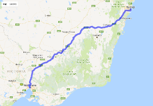
Melbourne to Sydney
The same query using the developers API generates the data in JSON
{
   "geocoded_waypoints" : [
      {
         "geocoder_status" : "OK",
         "place_id" : "ChIJ90260rVG1moRkM2MIXVWBAQ",
         "types" : [ "colloquial_area", "locality", "political" ]
      },
      {
         "geocoder_status" : "OK",
         "place_id" : "ChIJP3Sa8ziYEmsRUKgyFmh9AQM",
         "types" : [ "colloquial_area", "locality", "political" ]
      }
   ],
   "routes" : [
      {
         "bounds" : {
            "northeast" : {
               "lat" : -33.8660005,
               "lng" : 151.2176931
            },
            "southwest" : {
               "lat" : -37.8136598,
               "lng" : 144.8875036
            }
         },
         "copyrights" : "Map data ©2017 Google",
         "legs" : [
            {
               "distance" : {
                  "text" : "878 km",
                  "value" : 878208
               },
               "duration" : {
                  "text" : "8 hours 44 mins",
                  "value" : 31447
               },
               "end_address" : "Sydney NSW, Australia",
               "end_location" : {
                  "lat" : -33.8689894,
                  "lng" : 151.2091978
               },
               "start_address" : "Melbourne VIC, Australia",
               "start_location" : {
                  "lat" : -37.8136598,
                  "lng" : 144.9629147
               },
    ... etc
This result can be returned in R using the google_directions() function. By default the result will be coerced to the simplest R structure possible using jsonlite::fromJSON(). If you want the result in JSON set simplify = FALSE.
library(googleway)

key <- "your_api_key"
df <- google_directions(origin = "Melbourne, Australia",
                        destination = "Sydney, Australia",
                        key = key,
                        mode = "driving",
                        simplify = TRUE)
The data used to draw the route on the map is the overview_polyline. This string represents a sequence of lat/lon pairs, encoded using a lossy compression algorithm (https://developers.google.com/maps/documentation/utilities/polylinealgorithm) that allows you to store the series of coordinates as a single string.
You can extract the polyline manually
pl <- df$routes$overview_polyline$pointsOr use the direction_polyline() accessor
pl <- direction_polyline(df)
pl
# [1] "rqxeF_cxsZgr@xmCekBhMunGnWc_Ank@vBpyCqjAfbAqmBjXydAe{AoF{oEgTqjGur@ch@qfAhUuiCww@}kEtOepAtdD{dDf~BsgIuj@}tHi{C{bGg{@{rGsmG_bDbW{wCuTyiBajBytF_oAyaI}K}bEkqA{jDg^epJmbB{gC}v@i~D`@gkGmJ_kEojD_O{`FqvCetE}bGgbDm_BqpD}pEqdGiaBo{FglEg_Su~CegHw`Cm`Hv[mxFwaAisAklCuUgzAqmCalJajLqfDedHgyC_yHibCizK~Xo_DuqAojDshAeaEpg@g`Dy|DgtNswBcgDiaAgEqgBozB{jEejQ}p@ckIc~HmvFkgAsfGmjCcaJwwD}~AycCrx@skCwUqwN{yKygH}nF_qAgyOep@slIehDcmDieDkoEiuCg|LrKo~Eb}Bw{Ef^klG_AgdFqvAaxBgoDeqBwoDypEeiFkjBa|Ks}@gr@c}IkE_qEqo@syCgG{iEazAmeBmeCqvA}rCq_AixEemHszB_SisB}mEgeEenCqeDab@iwAmZg^guB}cCk_F_iAmkGsu@abDsoBylBk`Bm_CsfD{jFgrAerB{gDkw@{|EacB_jDmmAsjC{yBsyFaqFqfEi_Ei~C{yAmwFt{B{fBwKql@onBmtCq`IomFmdGueD_kDssAwsCyqDkx@e\\kwEyUstC}uAe|Ac|BakGpGkfGuc@qnDguBatBot@}kD_pBmmCkdAgkB}jBaIyoC}xAexHka@cz@ahCcfCayBqvBgtBsuDxb@yiDe{Ikt@c{DwhBydEynDojCapAq}AuAksBxPk{EgPgkJ{gA}tGsJezKbcAcdK__@uuBn_AcuGsjDwvC_|AwbE}~@wnErZ{nGr_@stEjbDakFf_@clDmKkwBbpAi_DlgA{lArLukCBukJol@w~DfCcpBwnAghCweA}{EmyAgaEbNybGeV}kCtjAq{EveBwuHlb@gyIg\\gmEhBw{G{dAmpHp_@a|MsnCcuGy~@agIe@e`KkoA}lBspBs^}sAmgIdpAumE{Y_|Oe|CioKouFwuIqnCmlDoHamBiuAgnDqp@yqIkmEqaIozAohAykDymA{uEgiE}fFehBgnCgrGmwCkiLurBkhL{jHcrGs}GkhFwpDezGgjEe_EsoBmm@g}KimLizEgbA{~DwfCwvFmhBuvBy~DsqCicBatC{z@mlCkkDoaDw_BagA}|Bii@kgCpj@}{E}b@cuJxQwkK}j@exF`UanFzM{fFumB}fCirHoTml@CoAh`A"
Having retrieved the polyline, you can decode it into latitude and longitude coordinates using decode_pl().
polyline <- "rqxeF_cxsZgr@xmCekBhMunGnWc_Ank@vBpyCqjAfbAqmBjXydAe{AoF{oEgTqjGur@ch@qfAhUuiCww@}kEtOepAtdD{dDf~BsgIuj@}tHi{C{bGg{@{rGsmG_bDbW{wCuTyiBajBytF_oAyaI}K}bEkqA{jDg^epJmbB{gC}v@i~D`@gkGmJ_kEojD_O{`FqvCetE}bGgbDm_BqpD}pEqdGiaBo{FglEg_Su~CegHw`Cm`Hv[mxFwaAisAklCuUgzAqmCalJajLqfDedHgyC_yHibCizK~Xo_DuqAojDshAeaEpg@g`Dy|DgtNswBcgDiaAgEqgBozB{jEejQ}p@ckIc~HmvFkgAsfGmjCcaJwwD}~AycCrx@skCwUqwN{yKygH}nF_qAgyOep@slIehDcmDieDkoEiuCg|LrKo~Eb}Bw{Ef^klG_AgdFqvAaxBgoDeqBwoDypEeiFkjBa|Ks}@gr@c}IkE_qEqo@syCgG{iEazAmeBmeCqvA}rCq_AixEemHszB_SisB}mEgeEenCqeDab@iwAmZg^guB}cCk_F_iAmkGsu@abDsoBylBk`Bm_CsfD{jFgrAerB{gDkw@{|EacB_jDmmAsjC{yBsyFaqFqfEi_Ei~C{yAmwFt{B{fBwKql@onBmtCq`IomFmdGueD_kDssAwsCyqDkx@e\\kwEyUstC}uAe|Ac|BakGpGkfGuc@qnDguBatBot@}kD_pBmmCkdAgkB}jBaIyoC}xAexHka@cz@ahCcfCayBqvBgtBsuDxb@yiDe{Ikt@c{DwhBydEynDojCapAq}AuAksBxPk{EgPgkJ{gA}tGsJezKbcAcdK__@uuBn_AcuGsjDwvC_|AwbE}~@wnErZ{nGr_@stEjbDakFf_@clDmKkwBbpAi_DlgA{lArLukCBukJol@w~DfCcpBwnAghCweA}{EmyAgaEbNybGeV}kCtjAq{EveBwuHlb@gyIg\\gmEhBw{G{dAmpHp_@a|MsnCcuGy~@agIe@e`KkoA}lBspBs^}sAmgIdpAumE{Y_|Oe|CioKouFwuIqnCmlDoHamBiuAgnDqp@yqIkmEqaIozAohAykDymA{uEgiE}fFehBgnCgrGmwCkiLurBkhL{jHcrGs}GkhFwpDezGgjEe_EsoBmm@g}KimLizEgbA{~DwfCwvFmhBuvBy~DsqCicBatC{z@mlCkkDoaDw_BagA}|Bii@kgCpj@}{E}b@cuJxQwkK}j@exF`UanFzM{fFumB}fCirHoTml@CoAh`A"

df <- decode_pl(polyline)
head(df)
## lat lon
## 1 -37.81418 144.9632
## 2 -37.80598 144.9404
## 3 -37.78867 144.9380
## 4 -37.74520 144.9341
## 5 -37.73494 144.9270
## 6 -37.73554 144.9023And, of course, to encode a series of lat/lon coordinates you use encode_pl()
## [1] "pqxeF}bxsZer@vmCgkBlMunGjWc_Apk@vBpyCqjAfbAqmBjXydAg{AoFyoEgTojGsr@gh@sfAhUuiCuw@}kEtOepAvdD{dDd~BsgIuj@{tHi{C{bGg{@{rGsmGabDbW{wCuTwiBajBytFaoA{aI{K{bEkqA{jDg^gpJkbB{gC_w@g~D`@ikGmJ_kEojD_O}`FqvCctE}bGgbDk_BspD_qEodGgaBo{FilEi_Su~CcgHw`Cm`Hv[mxFwaAisAklCuUgzAsmCalJajLqfDcdHgyCayHibCezK~Xo_DuqAqjDshAeaEpg@g`Dy|DgtNqwBegDkaAeEogBozB{jEejQ_q@ckIc~HkvFkgAufGmjCcaJwwD}~AycCrx@skCwUqwN}yKygH}nF}pAgyOep@qlIghDemDgeDkoEkuCc|LtKq~E`}Bw{Ef^klG}@gdFsvAcxBeoDcqByoDypEciFkjBc|Ku}@gr@a}IkE_qEoo@syCgG}iEczAkeBmeCqvA}rCq_AgxEgmHszB}RksB}mEgeEgnCoeD_b@iwAmZi^guB}cCm_F_iAikGsu@cbDsoB{lBk`Bi_CsfD}jFerAgrB{gDiw@}|EacB_jDkmAsjC}yBsyFaqFofEk_Ei~C{yAowFv{ByfBwKsl@onBktCq`IqmFmdGueDakDssAssCyqDmx@e\\kwEyUstC}uAe|Ac|BakGpGmfGuc@mnDguBctBmt@}kDapBmmCkdAgkB}jBcIyoC}xAexHia@cz@ahCafCayBqvBitBuuDzb@wiDe{Imt@e{DwhBwdEynDqjCapAo}AuAmsBzPi{EiPgkJ{gA}tGsJezKbcAcdK__@wuBn_AauGsjDwvC_|AybE{~@unEpZ{nGt_@stEhbDakFh_@elDoKiwBdpAi_DjgAylArLykCDukJql@u~DfCepBwnAghCweA{{EmyAgaEbN{bGcV{kCrjAq{EveByuHlb@eyIg\\gmEhBw{GydAopHn_@_|MsnCcuGw~@agIg@e`KkoA}lBspBu^}sAmgIfpAsmE}Ya|Oc|CgoKouFwuIsnCmlDmHamBkuAinDop@wqIkmEsaIqzAmhAwkD{mA}uEciE}fFghBenCirGowCgiLsrBmhL}jHerGs}GihFupDezGgjEg_EuoBim@g}KmmLizEebAy~DwfCyvFmhBuvBy~DsqCicBatC{z@klCkkDqaDw_BagA}|Bii@kgCpj@}{E{b@cuJxQwkK}j@exF~TanFzM{fFumB_gCirHmTml@AoAd`A"Google Distance API
The Google Maps Distance API is a service that provides travel distance and time for a matrix of origins and destinations.
Finding the distances between Melbourne Airport, the MCG, a set of coordinates (-37.81659, 144.9841), to Portsea, Melbourne.
df <- google_distance(origins = list(c("Melbourne Airport, Australia"),
                                     c("MCG, Melbourne, Australia"),
                                     c(-37.81659, 144.9841)),
                      destinations = c("Portsea, Melbourne, Australia"),
                      key = key)

head(df)
$destination_addresses
[1] "Melbourne Rd, Victoria, Australia"

$origin_addresses
[1] "Melbourne Airport (MEL), Departure Dr, Melbourne Airport VIC 3045, Australia"
[2] "Jolimont Station, Wellington Cres, East Melbourne VIC 3002, Australia"
[3] "176 Wellington Parade, East Melbourne VIC 3002, Australia"

$rows
                                                        elements
1 130 km, 129501, 1 hour 38 mins, 5853, 1 hour 36 mins, 5770, OK
2 104 km, 104393, 1 hour 20 mins, 4819, 1 hour 20 mins, 4792, OK
3 104 km, 104350, 1 hour 20 mins, 4814, 1 hour 20 mins, 4788, OK

$status
[1] "OK"
Google Elevation API
The Google Maps Elevation API provides elevation data for all locations on the surface of the earth, including depth locations on the ocean floor (which return negative values).
Finding the elevation of 20 points between the MCG, Melbourne and the beach at Elwood, Melbourne
google_elevation(df_locations = data.frame(lat = c(-37.81659, -37.88950),
                                           lon = c(144.9841, 144.9841)),
                  location_type = "path",
                  samples = 20,
                  key = key,
                  simplify = TRUE)

$results
    elevation location.lat location.lng resolution
1  20.8899250    -37.81659     144.9841   9.543952
2   7.8955822    -37.82043     144.9841   9.543952
3   8.4334993    -37.82426     144.9841   9.543952
4   5.4820895    -37.82810     144.9841   9.543952
5  33.5920677    -37.83194     144.9841   9.543952
6  30.4819584    -37.83578     144.9841   9.543952
7  15.0097895    -37.83961     144.9841   9.543952
8  10.9842978    -37.84345     144.9841   9.543952
9  13.8762951    -37.84729     144.9841   9.543952
10 13.4834013    -37.85113     144.9841   9.543952
11 13.3473139    -37.85496     144.9841   9.543952
12 24.9176636    -37.85880     144.9841   9.543952
13 16.7720604    -37.86264     144.9841   9.543952
14  5.8330226    -37.86648     144.9841   9.543952
15 10.7889471    -37.87031     144.9841   9.543952
16  6.9589133    -37.87415     144.9841   9.543952
17  3.9915009    -37.87799     144.9841   9.543952
18  5.3637657    -37.88183     144.9841   9.543952
19  7.1594319    -37.88566     144.9841   9.543952
20  0.6697893    -37.88950     144.9841   9.543952

$status
[1] "OK"
Google Timezone API
The Google Maps Time zone API provides time offset data for locations on the surface of the earth. You request the time zone information for a specific latitude/longitude pair and date. The API returns the name of that time zone, the time offset from UTC, and the daylight savings offset.
Finding the timezone of the MCG in Melbourne
google_timezone(location = c(-37.81659, 144.9841),
                timestamp = as.POSIXct("2016-06-05"),
                key = key,
                simplify = FALSE)

[1] "{"
[2] "   \"dstOffset\" : 0,"
[3] "   \"rawOffset\" : 36000,"
[4] "   \"status\" : \"OK\","
[5] "   \"timeZoneId\" : \"Australia/Hobart\","
[6] "   \"timeZoneName\" : \"Australian Eastern Standard Time\""
[7] "}"
Google Geocode API
The Google Maps Geocoding API is a service that provides geocoding and reverse geocoding of addresses.
Finding the location details for Flinders Street Station, Melbourne
df <- google_geocode(address = "Flinders Street Station",
                     key = key,
                     simplify = TRUE)

df$results$formatted_address
[1] "Flinders St, Melbourne VIC 3000, Australia"

## If your search responde multiple results, you can
## bound the search, for example

bounds <- list(c(-37.81962,144.9657),
               c(-37.81692, 144.9684))

df <- google_geocode(address = "Flinders Street Station",
                     bounds = bounds,
                     key = key,
                     simplify = TRUE)

## (in this example only one result was returned in the original call)
The coordinates of the location can be accessed with
geocode_coordinates(df)
#         lat      lng
# 1 -37.81827 144.9671
Google Reverse Geocode API
The Google Maps Reverse Geocoding API is a service that converts geographic coordinates into a human-readable address.
Finding the street address for a set of coordinates, using result_type and location_type as bounding parameters:
df <- google_reverse_geocode(location = c(-37.81659, 144.9841),
                             result_type = c("street_address", "postal_code"),
                             location_type = "rooftop",
                             key = key,
                             simplify = TRUE)

df$results$address_components
[[1]]
          long_name        short_name                                  types
1               176               176                          street_number
2 Wellington Parade Wellington Parade                                  route
3    East Melbourne    East Melbourne                    locality, political
4          Victoria               VIC administrative_area_level_1, political
5         Australia                AU                     country, political
6              3002              3002                            postal_code

df$results$geometry
  location.lat location.lng location_type viewport.northeast.lat viewport.northeast.lng viewport.southwest.lat
1    -37.81608     144.9842       ROOFTOP              -37.81473               144.9855              -37.81743
  viewport.southwest.lng
1               144.9828
Google Places API
The Google Maps Places API gets data from the same database used by Google Maps and Google+ Local. Places features more than 100 million businesses and points of interest that are updated frequently through owner-verified listings and user-moderated contributions.
There are three types of search you can perform
- Nearby
- Text
- Place Details
A Nearby Search lets you search for places within a specified area. You can refine your search request by supplying keywords or specifying the type of place you are searching for.
A Text Search Service is a web service that returns information about a set of places based on a string — for example “pizza in New York” or “shoe stores near Ottawa” or “123 Main Street”. The service responds with a list of places matching the text string and any location bias that has been set.
A Place Detail search (using google_place_details()) can be performed when you have a given place_id from one of the other three search methods.
Text
For a text search you are required to provide a search_string
For example, here’s a query for “restaurants in Melbourne”
res <- google_places(search_string = "Restaurants in Melbourne, Australia",
                     key = key)

## View the names of the returned restaurantes, and whether they are open or not

cbind(res$results$name, res$results$opening_hours)

                                            res$results$name open_now weekday_text
1                                               Vue de monde     TRUE         NULL
2                                                      ezard    FALSE         NULL
3                                                     MoVida     TRUE         NULL
4                           Flower Drum Restaurant Melbourne     TRUE         NULL
5                                             The Press Club    FALSE         NULL
6                                                       Maha     TRUE         NULL
7                                                  Bluestone       NA         NULL
8                                                  Chin Chin     TRUE         NULL
9                                               Taxi Kitchen     TRUE         NULL
10                                           Max on Hardware     TRUE         NULL
11                                                    Attica    FALSE         NULL
12                                       Nirankar Restaurant    FALSE         NULL
13                                                  The Mill     TRUE         NULL
14                                   The Left Bank Melbourne     TRUE         NULL
15                           The Colonial Tramcar Restaurant     TRUE         NULL
16                                      Rockpool Bar & Grill     TRUE         NULL
17 Lane Restaurant Cafe & Bar - Novotel Melbourne on Collins     TRUE         NULL
18                                          Melba Restaurant     TRUE         NULL
19                                              CUMULUS INC.     TRUE         NULL
20                                    radii restaurant & bar    FALSE         NULL
A single query will return 20 results per page. You can view the next 20 results using the next_page_token that is returned as part of the initial query.
res_next <- google_places(search_string = "Restaurants in Melbourne, Australia",
                          page_token = res$next_page_token,
                          key = key)

cbind(res_next$results$name, res_next$results$opening_hours)

                     res_next$results$name open_now weekday_text
1  Moshi Moshi Japanese Seafood Restaurant     TRUE         NULL
2                      Grill Steak Seafood     TRUE         NULL
3                             Conservatory     TRUE         NULL
4                                    Sarti    FALSE         NULL
5                                  Tsindos     TRUE         NULL
6                 The Cerberus Beach House     TRUE         NULL
7                   Stalactites Restaurant     TRUE         NULL
8            Hanabishi Japanese Restaurant    FALSE         NULL
9                          GAZI Restaurant     TRUE         NULL
10                           Om Vegetarian    FALSE         NULL
11                           Shark Fin Inn     TRUE         NULL
12                           Om Vegetarian     TRUE         NULL
13                 The Atlantic Restaurant     TRUE         NULL
14                                  Takumi     TRUE         NULL
15                              Pei Modern       NA         NULL
16                 Bamboo House Restaurant     TRUE         NULL
17                 Byblos Bar & Restaurant     TRUE         NULL
18                              Waterfront     TRUE         NULL
19                                   No 35     TRUE         NULL
20                        Bistro Guillaume     TRUE         NULL
Nearby
For a nearby search you are required to provide a location as a pair of latitude/longitude coordinates. You can refine your search by providing a keyword and / or a radius.
res <- google_places(location = c(-37.918, 144.968),
                    keyword = "Restaurant",
                    radius = 5000,
                    key = key)


cbind(res$results$name, res$results$opening_hours)
#                         res$results$name open_now weekday_text
# 1                              Melbourne       NA         NULL
# 2              Quest Brighton on the Bay     TRUE         NULL
# 3                         Brighton Savoy    FALSE         NULL
# 4  Caroline Serviced Apartments Brighton     TRUE         NULL
# 5      The Buckingham Serviced Apartment       NA         NULL
# 6                      Sandringham Hotel     TRUE         NULL
# 7               Indian Palace Restaurant     TRUE         NULL
# 8                       Elsternwick Park     TRUE         NULL
# 9                         Brown Cow Cafe     TRUE         NULL
# 10              Bok Choy Chinese Cuisine    FALSE         NULL
# 11                          Marine Hotel     TRUE         NULL
# 12                          Daily Planet     TRUE         NULL
# 13                         Riva St Kilda     TRUE         NULL
# 14                         New Bay Hotel     TRUE         NULL
# 15          Flight Centre North Brighton     TRUE         NULL
# 16              Vintage Cellars Brighton     TRUE         NULL
# 17                   Palace Brighton Bay     TRUE         NULL
# 18                       Brighton Toyota     TRUE         NULL
# 19                            Sportsgirl     TRUE         NULL
# 20                           Saint Kilda       NA         NULL
Google Roads
The Google Roads API provides three functions
- Snap To Roads
- Nearest Roads
- Speed Limits (premium only)
Snap to Roads
The snap to roads function takes up to 100 GPS points collected along a route and returns the points snapped to the most likely roads that were travelled along.
df_path <- read.table(text = "lat lon
-35.27801 149.12958
-35.28032 149.12907
-35.28099 149.12929
-35.28144 149.12984
-35.28194 149.13003
-35.28282 149.12956
-35.28302 149.12881
-35.28473 149.12836
", header = T, stringsAsFactors = F)


res <- google_snapToRoads(df_path = df_path, key = key)

res$snappedPoints
  location.latitude location.longitude originalIndex                     placeId
1         -35.27800           149.1295             0 ChIJr_xl0GdNFmsRsUtUbW7qABM
2         -35.28032           149.1291             1 ChIJOyypT2hNFmsRZBtscGL0htw
3         -35.28101           149.1292             2 ChIJv5r0smlNFmsR5nunau79Fv4
4         -35.28147           149.1298             3 ChIJ601MoWlNFmsR5mvkfPp2ovA
5         -35.28194           149.1300             4 ChIJ601MoWlNFmsR5mvkfPp2ovA
6         -35.28282           149.1296             5 ChIJaUpThGlNFmsRMHWxoH7EOsc
7         -35.28313           149.1289             6 ChIJWSb8ImpNFmsRp_4JAxJFE1A
8         -35.28473           149.1283             7 ChIJtWxAZmpNFmsRlbUCkc6VtnA
The result includes the column originalIndex. This is a zero-based index that indicates which of the input coordinates has been snapped to the given location.latitude/location.longitude coordinates. So in this example, originalIndex 0 is the first row of df_path, originalIndex 1 is the second row of df_path, and so on.
Nearest Roads
The nearest roads function takes up to 100 independent coordinates and returns the closest road segment for each point.
df_points <- read.table(text = "lat lon
60.1707 24.9426
60.1708 24.9424
60.1709 24.9423", header = T)

res <- google_nearestRoads(df_points, key = key)

res$snappedPoints
  location.latitude location.longitude originalIndex                     placeId
1          60.17070           24.94272             0 ChIJNX9BrM0LkkYRIM-cQg265e8
2          60.17081           24.94271             1 ChIJNX9BrM0LkkYRIM-cQg265e8
3          60.17091           24.94270             2 ChIJNX9BrM0LkkYRIM-cQg265e8
Google Maps
A google map can be made using the google_map() function. Without any data present, or no location value set, the map will default to Melbourne, Australia.
You can also display traffic, transit (public transport) or bicycle routes using the functions add_traffic(), add_transit() and add_bicycling() respectively.
You can also include a search box in your map by using the argument search_box = TRUE, which allows you to search the maps just like you would when using Google Maps.
map_key <- "your_api_key"
google_map(key = map_key, search_box = T) %>%
  add_traffic()
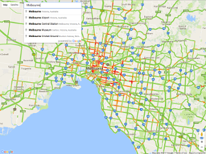
Melbourne
Markers
Markers and circles can be used to show points on the map.
In this example I’m using the tram_stops data set provided with googleway.
You can specify a column in the data.frame to use to populate a popup info_window that will be displayed when clicking on a maker. The info window can display any valid HTML, as demonstrated in this Stack Overflow answer.
df <- tram_stops
df$info <- paste0("<b>Stop Name: </b>", df$stop_name)

map_key <- "your_api_key"
google_map(data = df, key = map_key) %>%
  add_markers(lat = "stop_lat", lon = "stop_lon", info_window = "info")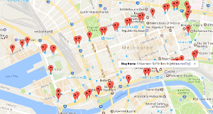
Marker Info Window
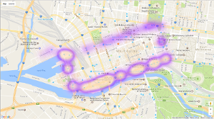
Heatmap
You can create a heatmap using Google’s Heatlayer.
google_map(data = tram_stops, key = map_key) %>%
  add_heatmap(lat = "stop_lat", lon = "stop_lon", option_radius = 0.0025)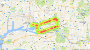
Heatmap
There are a few options you can configure to change how the heatmap is plotted, for example changing the colours, and weight associated with each point in the data set
## the colours can be any of those given by colors()
tram_stops$weight <- 1:nrow(tram_stops)

google_map(data = tram_stops, key = map_key) %>%
  add_heatmap(lat = "stop_lat", lon = "stop_lon", option_radius = 0.0025,
              weight = 'weight',
              option_gradient = c("plum1", "purple1", "peachpuff"))
Heatmap Colour
Polyline
Polylines in Google Maps are formed from a set of latitude/longitude coordinates, encoded into a polyline string.
Both the add_polylines() and add_polygons() functions in googleway can plot the encoded polyline to save the amount of data set to the browser. (They can also plot coordinates, but this is often slower).
To draw a line on a map you use the add_polylines() function. This function takes a data.frame with at least one column of data containing the polylines, or two columns containing the series of lat/lon coordinates.
Here we can plot the polyline we generated earlier from querying the directions from Melbourne to Sydney.
df <- data.frame(polyline = pl)

google_map(key = map_key) %>%
    add_polylines(data = df, polyline = "polyline", stroke_weight = 9)
Polyline
Polygon
A polygon represents an area enclosed by one or more polylines. Holes are denoted by defining an inner path wound in the opposite direction to the outer path.
To draw a polygon on a map use the add_polygons() function. This function takes a data.frame, where the polygons can be specified in one of three ways
- Multiple rows of latitude and longitude coordinates that specify paths, using an
idandpathIdvalue to specify the polygon that each path belongs to - Rows of encoded polylines, using a
idvalue to specify the polygon that each polyline represents - Rows of nested polylines in a list column. Each row represents a polygon, and each polyline in the list represents the paths that make up the polygon.
The melbourne data set provided with googleway is a data.frame of polygons of Melbourne and the surrounding suburbs. The coordinates of the polygons are encoded in to polylines.
##     polygonId pathId     SA2_NAME             SA3_NAME
## 386       338      1 Point Nepean Mornington Peninsula
## 387       338      2 Point Nepean Mornington Peninsula
##                 SA4_NAME AREASQKM               polyline
## 386 Mornington Peninsula  67.1875 `haiFgzjrZJMJBBRIJMCCQ
## 387 Mornington Peninsula  67.1875 z{biFyqlrZARO@SUTOB@JL
Plotting this data is done using add_polygons()
google_map(key = "your_api_key") %>%
  add_polygons(data = melbourne, polyline = "polyline", fill_colour = "SA4_NAME")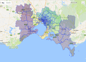
Melbourne Polygons
In this example I’ve specified the fill_colour to be one of the columns of the melbourne data set. The plotting functions in googleway will map the variables in the column to a given colour. The default colour scale is taken from viridisLite::viridis().
Colours & Legend
Where applicable the map layer functions provide two arguments that you can use to plot colours
-
fill_colour(for colouring an area) -
stroke_colour(for colouring a line / outline of an area)
Each of those arguments can be mapped to a column of data (as in the Polygon example), or if you want to use your own colours you can either
- specify the palette using the
paletteargument
google_map(key = "your_api_key") %>%
  add_polygons(data = melbourne, polyline = "polyline", fill_colour = "SA4_NAME", palette = viridisLite::inferno)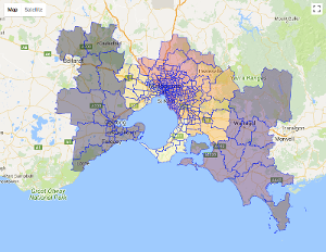
Colour Palette
- add a column of hex colour values and supply this to the plotting function
colours <- RColorBrewer::brewer.pal(9, "Set1")
melbourne$randomColour <- sample(colours, size = nrow(melbourne), replace = T)
google_map(key = "your_api_key") %>%
  add_polygons(data = melbourne, polyline = "polyline", fill_colour = "randomColour")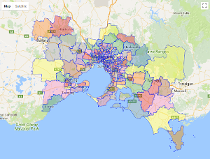
Colour Column
- specify a single hex colour value to either
fill_colourorstroke_colourto colour all shapes the same colour
google_map(key = "your_api_key") %>%
  add_polygons(data = melbourne, polyline = "polyline", fill_colour = "#FF00FF")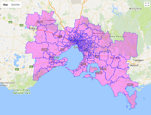
Single Colour
Setting legend = TRUE will give you a legend
google_map(key = "your_api_key") %>%
  add_polygons(data = melbourne, polyline = "polyline", fill_colour = "SA4_NAME", legend = T)
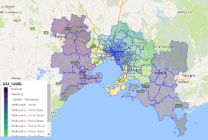
Legend
You can customise the legend by supplying any of the arguments in a list to the legend_options argument
- position - one of TOP_LEFT, TOP_CENTER, TOP_RIGHT, RIGHT_TOP, RIGHT_CENTER, RIGHT_BOTTOM, BOTTOM_RIGHT, BOTTOM_CENTER, BOTTOM_LEFT, LEFT_BOTTOM, LEFT_CENTER and LEFT_TOP
- css - a string of valid CSS for controlling the appearance
- title - a string to use for the title of the legend. The default is the column name mapped to the colour
If you are displaying two legends, one for stroke_colour and one for fill_colour, you can specify different options for the different colour attributes
legendOpts <- list(
  fill_colour = list(position = "TOP_RIGHT"),
  stroke_colour = list(position = "BOTTOM_LEFT", title = "SA3")
  )

google_map(key = "your_api_key") %>%
  add_polygons(data = melbourne, polyline = "polyline", fill_colour = "SA4_NAME", stroke_colour = "SA3_NAME", legend = T, legend_options = legendOpts)
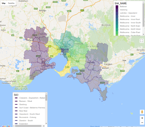
Custom Legend
Simple Features
googleway supports plotting certain geometries from sf objects (from library(sf))
- POINT and MULTIPOINT plotted with
add_markers()andadd_circles() - LINESTRING and MULTILINESTRING plotted with
add_polylines() - POLYGON and MULTIPOLYGON plotted with
add_polygons()
This example uses and plots the polygons from the North Carolina data set supplied with library(sf)
library(sf)
nc <- sf::st_read(system.file("shape/nc.shp", package="sf"))

google_map(data = nc) %>%
  add_polygons()
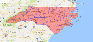
sf North Carolina
If the sf objects contains multiple geometries, you can also use the various add_* functions to add specific rows of the sf object. The mapping between the functions and the sf objects is
-
add_markers()- POINT & MULTIPOINT -
add_circles()- POINT & MULTIPOINT -
add_polylines()- LINESTRING & MULTILINESTRING -
add_polygons()- POLYGON & MULTIPOLYGON
df <- data.frame(myId = c(1,1,1,1,1,1,1,1,2,2,2,2),
  lineId = c(1,1,1,1,2,2,2,2,1,1,1,2),
    lon = c(-80.190, -66.118, -64.757, -80.190,  -70.579, -67.514, -66.668, -70.579, -70, -49, -51, -70),
    lat = c(26.774, 18.466, 32.321, 26.774, 28.745, 29.570, 27.339, 28.745, 22, 23, 22, 22))

p1 <- as.matrix(df[4:1, c("lon", "lat")])
p2 <- as.matrix(df[8:5, c("lon", "lat")])
p3 <- as.matrix(df[9:12, c("lon", "lat")])

point <- sf::st_sfc(sf::st_point(x = c(df[1,"lon"], df[1,"lat"])))
multipoint <- sf::st_sfc(sf::st_multipoint(x = as.matrix(df[1:2, c("lon", "lat")])))
polygon <- sf::st_sfc(sf::st_polygon(x = list(p1, p2)))
linestring <- sf::st_sfc(sf::st_linestring(p3))
multilinestring <- sf::st_sfc(sf::st_multilinestring(list(p1, p2)))
multipolygon <- sf::st_sfc(sf::st_multipolygon(x = list(list(p1, p2), list(p3))))

sf <- rbind(
    sf::st_sf(geometry = polygon),
    sf::st_sf(geometry = multipolygon),
    sf::st_sf(geometry = multilinestring),
    sf::st_sf(geometry = linestring),
    sf::st_sf(geometry = point),
  sf::st_sf(geometry = multipoint)
)


google_map(data = sf) %>%
  add_markers() %>%
  add_polylines()
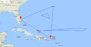
sf marker & line
GeoJSON
The geo_melbourne data set is a GeoJSON representation of a subset of the melbourne data set. You can use add_geojson to plot this data
google_map() %>%
  add_geojson(data = geo_melbourne)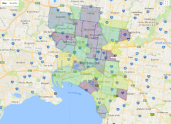
Geojson
By default add_geojson() will apply any styles included in the GeoJSON file. In the geo_melbourne data you can see the styles fillColor, strokeColor and strokeWeight
## [1] "{\"type\":\"FeatureCollection\",\"features\":[{\"type\":\"Feature\",\"properties\":{\"SA2_NAME\":\"Abbotsford\",\"polygonId\":70,\"SA3_NAME\":\"Yarra\",\"AREASQKM\":1.7405,\"fillColor\":\"#440154\",\"strokeColor\":\"#440154\",\"strokeWeight\":1},\"geometry\":{\"type\":\"Polygon\",\"coordinates\":[[[144.9925232,-37.8024902],[144.9926453,-37."You can also supply a string of JSON to style all the features in the GeoJSON
style <- '{ "fillColor" : "green" , "strokeColor" : "black", "strokeWeight" : 0.5}'
google_map(key = "your_api_key") %>%
  add_geojson(data = geo_melbourne, style = style)
Or you can use a named list to have the same effect
style <- list(fillColor = "red" , strokeColor = "blue", strokeWeight = 0.5)
google_map(key = "your_api_key") %>%
  add_geojson(data = geo_melbourne, style = style)
Drag & Drop Geojson
The function add_dragdrop() creates a map on to which you can drag & drop a GeoJSON file. There is an example of this in action on my blog
Rectangles
Rectangles can be added by supplying north, east, south and west coordinates to add_rectangles()
df <- data.frame(north = 33.685, south = 33.671, east = -116.234, west = -116.251)

google_map(key = "your_api_key") %>%
  add_rectangles(data = df, north = 'north', south = 'south',
                 east = 'east', west = 'west')
Drawing
You can create your own shapes on a map using add_drawing(). The shapes you can create are
- markers
- circles
- polygon
- polyline
- rectangle
This can be particularly useful when working with shiny as the shape information can be returned when drawing is completed.
For example, use the following code to create a shiny that enables drawing circles.
library(shiny)

ui <- fluidPage(
  google_mapOutput(outputId = "map", height = "800px")
)

server <- function(input, output){

  mapKey <- "your_map_key"
  output$map <- renderGoogle_map({
    google_map(key = mapKey) %>%
      add_drawing(drawing_modes = c("circle"))
  })


  observeEvent(input$map_circlecomplete, {
    print(input$map_circlecomplete)
  })
}
shinyApp(ui, server)
When a circle is drawin, the print(input$map_circlecomplete) function prints the following information to the console (it will vary based on where you draw the circle)
$center
$center$lat
[1] -36.80489

$center$lng
[1] 144.2889


$radius
[1] 57970.9

$bounds
$bounds$south
[1] -37.32565

$bounds$west
[1] 143.6385

$bounds$north
[1] -36.28413

$bounds$east
[1] 144.9393


$randomValue
[1] 0.3688953
Fusion Layers
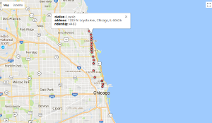
The fusion layer renders data contained in a Google Fusion Table. At the time of writing the Fusion Layer is still experimental.
A Google Fusion Table is a database table where each row contains data about a particular feature; for geographic data, each row within a Google Fusion Table additionally contains location data, holding a feature’s positional information. The FusionTablesLayer provides an interface to Fusion Tables and supports automatic rendering of this location data, providing clickable overlays that display a feature’s additional data.
To add a fusion layer you need to query the table using least a select and a from property. The query must be supplied in a data.frame or a JSON string. If a data.frame is used it must be one row long, and either 2 or 3 columns.
qry <- data.frame(select = 'address',
    from = '1d7qpn60tAvG4LEg4jvClZbc1ggp8fIGGvpMGzA',
    where = 'ridership > 200')

## Or as a list
# qry <- list(select = 'address',
#     from = '1d7qpn60tAvG4LEg4jvClZbc1ggp8fIGGvpMGzA',
#     where = 'ridership > 200')

google_map(key = "your_api_key", location = c(41.8, -87.7), zoom = 9) %>%
  add_fusion(query = qry)
Fusion Layer
You can also supply a styles argument to style the layers
## Query using a JSON string
qry <- '{"select":"geometry","from":"1ertEwm-1bMBhpEwHhtNYT47HQ9k2ki_6sRa-UQ"}'

styles <- '[
  {
    "polygonOptions":{
      "fillColor":"#FFFF00",
      "fillOpacity":0.3
      }
    },
    {
      "where":"birds > 300",
       "polygonOptions":{
         "fillColor":"#000000"
       }
     },
     {
       "where":"population > 5",
       "polygonOptions":{
         "fillOpacity":1
         }
     }
   ]'

google_map(key = "your_api_key", location = c(-25.3, 133), zoom = 4) %>%
  add_fusion(query = qry, styles = styles)


## The style will also work as a JSON object
# attr(styles, 'class') <- 'json'
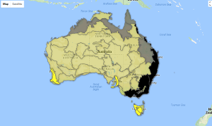
Fusion Styles
KML & GeoRSS
The add_kml() function renders KML and GeoRSS elements on a Google Map. All you need to specify is a URL containing the kml data.
kmlUrl <- 'http://googlemaps.github.io/js-v2-samples/ggeoxml/cta.kml'

google_map(key = "your_api_key") %>%
  add_kml(kml_url = kmlUrl)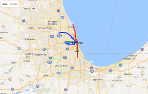
KML
Overlays
Overalys are objects on the map that are tied to latitude/longitude coordinates, so they move when you drag or zoom the map.
You need to supply the lat/lon coordinates to the north (lat), south (lat), east (lon) and west (lon) arguments, and a URL to the overlay.
google_map(key = "your_api_key") %>%
  add_overlay(north = 40.773941, south = 40.712216, east = -74.12544, west = -74.22655,
               overlay_url = "https://www.lib.utexas.edu/maps/historical/newark_nj_1922.jpg")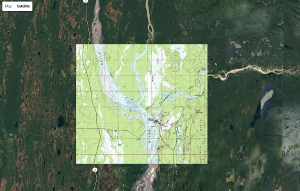
Overlay
Shiny
As google_map() is an HTMLWidget, it inherently works in Shiny. As with all shiny apps the two functions you need to include are
-
renderGoogle_map()(in the UI) -
google_mapOutput()(in the server)
The simplest app can be built with
library(shiny)

ui <- fluidPage(
   google_mapOutput(outputId = "map")
)

server <- function(input, output){

  map_key <- 'your_api_key'

  output$map <- renderGoogle_map({
    google_map(key = map_key)
  })
}

shinyApp(ui, server)
But, of course, this isn’t very interesting.
You can use all the standard add_* functions that have already been discussed to add various shapes and layers. But there’s also various clear_* and update_* functions that let you update those shapes and layers dynamically within the shiny app.
The clear_* functions are designed to remove objects from the app.
The update_* functions are designed to update those objects that are already on the map. This is useful for when you want to update existing polylines, polygons, rectangles, circles and markers.
library(shiny)

ui <- fluidPage(
  sliderInput(inputId = "opacity", label = "opacity", min = 0, max = 1,
              step = 0.01, value = 1),
  google_mapOutput(outputId = "map")
)

server <- function(input, output){

  map_key <- 'your_api_key'

  output$map <- renderGoogle_map({

    google_map(key = map_key) %>%
      add_polygons(data = melbourne, id = "polygonId", pathId = "pathId",
                   polyline = "polyline", fill_opacity = 1)
  })

  ## observe the opacity slider changing
  observeEvent(input$opacity, {

    melbourne$opacity <- input$opacity

    google_map_update(map_id = "map") %>%
      update_polygons(data = melbourne, fill_opacity = "opacity", id = "polygonId")
  })

}

shinyApp(ui, server)
Note that to use the udpate_* functions you need to provide the id of the object you want to update.
The exception to the update_* functions is update_heatmap(), which allows you to both add and remove points from the heat layer.
library(shiny)

ui <- fluidPage(
  sliderInput(inputId = "sample", label = "sample", min = 1, max = 10,
              step = 1, value = 10),
  google_mapOutput(outputId = "map")
)

server <- function(input, output){

  #map_key <- 'your_api_key'

  set.seed(20170417)
  df <- tram_route[sample(1:nrow(tram_route), size = 10 * 100, replace = T), ]

  output$map <- renderGoogle_map({
    google_map(key = map_key) %>%
      add_heatmap(data = df, lat = "shape_pt_lat", lon = "shape_pt_lon",
                  option_radius = 0.001)
  })

  observeEvent(input$sample,{

    df <- tram_route[sample(1:nrow(tram_route), size = input$sample * 100, replace = T), ]

    google_map_update(map_id = "map") %>%
      update_heatmap(data = df, lat = "shape_pt_lat", lon = "shape_pt_lon")
  })
}

shinyApp(ui, server)
Returning Data
One of the more powerful features of googleway mapping is the ability to return data from the maps to R using Shiny.
Data can be returned using
- clicking on the map
- panning / zooming the map
- shape / layer clicks
- editing shapes
- dragging shapes
Within the google_map() call you can pass one of two values to the event_return_type argument, “list” or “json”. This controls the type of data structure returned back to R from Shiny.
Clicking on the map
Data can be retrieved from the map by clicking on it and “observing” the clicks.
The structure of the observed event is
input$<map_id>_map_click
where
-
<map_id>is the id of the output map element (see example) -
map_clickis the event being observed
library(shiny)
ui <- fluidPage(
 google_mapOutput('myMap')
)
server <- function(input, output){
 output$myMap <- renderGoogle_map({
   google_map(key = "your_api_key", event_return_type = "list")
 })
 observeEvent(input$myMap_map_click, {
    print(input$myMap_map_click)
 })
}
shinyApp(ui, server)
Clicking on the map in this example will return the following fields
$id
[1] "myMap"

$lat
[1] -37.68382

$lon
[1] 145.08

$centerLat
[1] -37.9

$centerLon
[1] 144.5

$zoom
[1] 8

$randomValue
[1] 0.4043373
Similarly, observing input$myMap_bounds_changed will observe panning the map, and input$myMap_zoom_changed will observe zooming the map.
Shape / layer clicks
Data can be retrieved from shapes by clicking on them and “observing” the clicks.
The structure of the observed event is
input$<map_id>_<shape>_click
where
-
<map_id>is the id of the output map element (see example) -
<shape>is the shape being clicked (e.g. polygon, polyline, circle, etc) -
clickis the event being observed
library(shiny)
ui <- fluidPage(
 google_mapOutput('map')
)
server <- function(input, output){
 output$map <- renderGoogle_map({
   google_map(key = "your_api_key", event_return_type = "list") %>%
     add_polygons(data = melbourne, polyline = "polyline")
 })
 observeEvent(input$map_polygon_click, {
    print(input$map_polygon_click)
 })
}
shinyApp(ui, server)
Clicking on one of the polygons in this example will return the fields
$id
[1] 22

$lat
[1] -38.16911

$lon
[1] 144.6872

$outerPath
[1] "dlsgFyduq..." ## truncated

$allPaths
$allPaths[[1]]
[1] "dlsgFyduqZ..." ## truncated


$randomValue
[1] 0.5917599

$layerId
[1] "defaultLayerId"